The following chapter contain descriptions of legacy nodes which are no longer available in the GA3 Editor. Recipes created with version 5.4x may utilize such nodes. Therefore they are maintained in the software and also their descriptions are kept here:
Heatmap of a property related to grid type patterns (wellplate) where x, y axes are mapped into columns and rows.
Tracking results with fixed number of tracks and time points can color code speed or other track properties at given time.
Changes the bit-depth of the connected result.
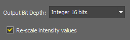
Figure 1048.
Sets a new color depth of your image. 8-bit/16-bit integer or a floating-point. Intensity values can be rescaled.
If checked the pixel values are mapped to the new range. E.g. when you convert an 8bit image to 16bit and you do not rescale the values, it results in a completely black image. If the check box was selected, the 8bit 255 value would become 65535 in 16bit etc.
Removes any binary object not meeting the specified condition. Objects having the specified feature outside of the specified range will be removed.
Transforms the source into the result with transformation programmed in JavaScript. Up to 6 binary/color/table inputs can be added.
See the dedicated documentation: Extending GA3.
Counts the number of objects in the connected binary result.
Counts the number of pixels (“TotalPixelCount”) in the connected binary result.
Area covered by the connected binary result (“TotalObjectArea”) is calculated.
Area of the connected binary result is divided by the total area of the analysed image (“AreaFraction”).
Displays the total area (“MeasuredArea”) of the currently analysed image.
Please see Perimeter.
Please see MeanChord.
Please see SurfVolumeRatio.
Calculates entropy of all pixel values in the color image. If the connected color image has multiple channels they are averaged into a single value per pixel. If a binary is connected only pixels under it are taken.
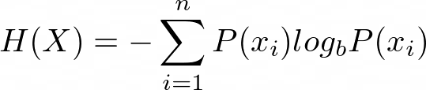
Figure 1049.
where P(X) is the distribution of intensity values.
Calculates the value defining which focus criterion is used. For more information please see Devices > Auto Focus Setup.
Calculates sample kurtosis of all pixel values in the color image. If the connected color image has multiple channels they are averaged into a single value per pixel. If a binary is connected only pixels under it are taken.
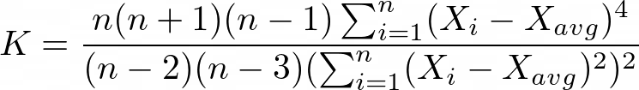
Figure 1050.
Calculates the maximal pixel intensity (“MaxIntensity”) of the connected color result under the connected binary result. Please see MaxIntensity.
Calculates arithmetic mean of all pixel values in the color image. If the connected color image has multiple channels they are averaged into a single value per pixel. If a binary is connected only pixels under it are taken.
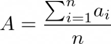
Figure 1051.
Calculates the minimal pixel intensity (“MinIntensity”) of the connected color result under the connected binary result. Please see MinIntensity.
Mode finds pixel value that appears most often in the color image. If the connected color image has multiple channels they are averaged into a single value per pixel. If a binary is connected only pixels under it are taken.
Calculates the value of Otsu's threshold. For more information please see Otsu's method.
Calculates the n-th quantile of all pixel values in the color image. If the connected color image has multiple channels they are averaged into a single value per pixel. If a binary is connected only pixels under it are taken.
Quantile is a cut point dividing the range of values of input into two parts such that the first part contains 100 * Quantile % of values and the second part contains 100 * (1 - Quantile) % of values. If the quantile is set to 0.5, this function computes the median of values.
This action fits a Gaussian curve to the pixel value density graph (histogram) using linear regression. If the connected color image has multiple channels they are averaged into a single value per pixel. It returns the following Gaussian curve parameters: Mean, Sigma, and R^2 (coeffiecient of determination representing the goodness of fit).
Equation of Gaussian curve:
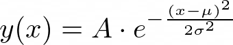
Figure 1052.
Calculates sample skewness of all pixel values in the color image. If the connected color image has multiple channels they are averaged into a single value per pixel. If a binary is connected only pixels under it are taken.
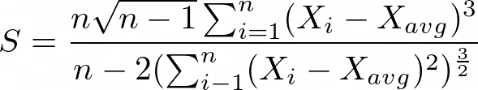
Figure 1053.
Calculates sample standard deviation of all pixel values in the color image. If the connected color image has multiple channels they are averaged into a single value per pixel. If a binary is connected only pixels under it are taken.
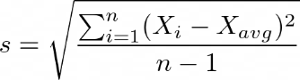
Figure 1054.
Calculates sum of all pixel values in the color image. If the connected color image has multiple channels they are averaged into a single value per pixel. If a binary is connected only pixels under it are taken.
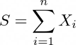
Figure 1055.
Calculates uniformity of all pixel values in the color image. If the connected color image has multiple channels they are averaged into a single value per pixel. If a binary is connected only pixels under it are taken.
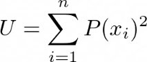
Figure 1056.
where P(X) is the distribution of intensity values.
Calculates sample variance of all pixel values in the color image. If the connected color image has multiple channels they are averaged into a single value per pixel. If a binary is connected only pixels under it are taken.
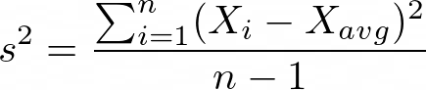
Figure 1057.
Calculates the mean of ratios between corresponding pixels of the two input channels under the input binary mask for the whole field.
Calculates Pearson correlation coefficient for the whole field. For more information please see Measurement > Object ratiometry > Pearson Coeff.
Calculates Manders overlap for the whole field. For more information please see Measurement > Object ratiometry > Manders Coeff.
Displays the acquisition time (“Time”) of the connected color result.
Displays the channel name of the connected source channel.
Returns basic metadata of each input channel component (Channel Name, Optical Configuration, Excitation Wavelength, Emission Wavelength, Modality, Magnification, Numerical Aparature, Immersion RI, Pinhole Size).
Returns the position of the frame center in micrometers.
Returns the position of the frame center in pixels.
Displays the frame size (“FrameSize.X” and “FrameSize.Y”) in [µm] of the image being processed.
Displays the frame size (“FrameSizePx.X” and “FrameSizePx.Y”) in pixels [px] of the image being processed.
Displays the maximum allowed pixel value (“MaxAllowedValue”) for the image being processed.
Displays the minimum allowed pixel value (“MinAllowedValue”) for the image being processed.
Gives access to the metadata such as Exposure Time, Plate Name, Well Row, Slide Barcode, etc.
Displays information about the stage position (“StagePos.X”, “StagePor.Y”, “StagePos.Z”) during acquisition of the image being processed.
Displays the Z Step size (“ZStep”) of the image being processed.
Calculates the Equivalent Diameter (“EqDiameter”) for each object in the connected binary result. It represents a circle with the same area as the measured object. For more information please see EqDiameter.
Calculates the Fill Area (“FillArea”) of each object in the connected binary result. Fill area calculation ignores any holes in the objects. For more information please see FillArea.
Calculates the length for each object in the connected binary result. Length is a derived feature appropriate for elongated or thin structures. Since it is based on the rod model, it is useful for calculating length of medial axis of thin rods. For more information please see Length.
Calculates the line length (“LineLength”) of each object in the connected binary result. For more information please see LineLength.
Calculates the maximal value of the set of Feret's diameters for each object in the connected binary result. For more information please see MaxFeret.
Calculates the length projected across the MaxFeret diameter for each object in the connected binary result. For more information please see MaxFeret90.
Calculates the minimal value of the set of Feret's diameters for each object in the connected binary result. For more information please see MinFeret.
Calculates the minimal rectangular area for each object in the connected binary result.
Counts the number of pixels in each binary object of the connected binary image.
Calculates the area of each object (“ObjectArea”) under the connected binary result.
Please see OuterPerimeter.
Please see Perimeter.
Please see PerimeterContour.
Please see VolumeEqCylinder.
Please see VolumeEqSphere.
Please see Width.
Please see Circularity.
Please see Convexity.
Please see Elongation.
Please see FillRatio.
Please see MeanChord.
Please see Orientation.
Calculates the rectangularity of each object of the connected binary image.
Please see Roughness.
Please see RoughnessInf.
Please see ShapeFactor.
Calculates entropy of the pixel values for every binary object.
Please see Measurement > Field intensity > Entropy.
Calculates sample kurtosis of the pixel values for every binary object.
Please see Measurement > Field intensity > Kurtosis.
Calculates the arithmetic mean of pixel values for every binary object.
Please see Measurement > Field intensity > Mean.
Finds pixel value that appears most often in every object.
Please see Measurement > Field intensity > Mode.
Calculates the n-th quantile of pixel values for every binary object.
Please see Measurement > Field intensity > Quantile.
Calculates the sample skewness of pixel values for every binary object.
Please see Measurement > Field intensity > Skewness.
Calculates the sample standard deviation of color pixel values for every binary object.
Please see Measurement > Field intensity > Standard Deviation.
Calculates the sum of pixel values for every binary object.
Please see Measurement > Field intensity > Sum.
Calculates the uniformity of pixel values for every binary object.
Please see Measurement > Field intensity > Uniformity.
Calculates the sample variance of pixel values for every binary object.
Please see Measurement > Field intensity > Variance.
Calculates the mean of ratios between corresponding pixels of the two input channels under the input binary mask.
Calculates Pearson correlation coefficient for pixels from two inputs (B, C) under input binary mask. The coefficient ranges from -1 to 1. A value of 1 implies positive linear relationship for which C increases as B increases. A value of -1 implies negative linear relationship for which C decreases as B increases. A value of 0 implies that there is no linear correlation between B and C.
Calculates Manders overlap (MOC), Manders overlap coefficients (k1, k2) and Manders colocalization coefficients (M1, M2).
See also View > Analysis Controls > Colocalization 
MOC - ranges from 0 to 1.
k1, k2 - range from 0 to oo. MOC^2 = k1 * k2
range from 0 to 1, where 1 implies perfect colocalization. They are not sensitive to intensity of overlapping pixels, but are very sensitive to background. A proper background subtraction step is necessary before measuring these coefficients.
is a fraction of R in areas containing G
is a fraction of G in areas containing R
Produces a table where each row represents parent object containing ParentEntity, ParentId, parent features (taken as input table), ChildId, aggregated (specified in the GUI) child features (taken as input table). Parent[Entity, Id] and Child[Entity, Id] are replaced with the name of the Binary.
couples each child to the parent object which completely covers it (child is completely inside its parent).
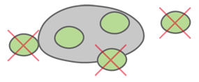
Figure 1058. Ignored objects are crossed out in red.
couples each child to the parent object which completely covers it or intersects with it. If a child intersects more than one parent, it belongs to the parent with which it has a bigger intersection.
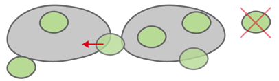
Figure 1059. Ignored objects are crossed out in red. Arrow indicates to which parent the child belongs.
couples each child to its nearest parent object. If a child lies on the border between two parent areas, it belongs to the parent with which area it has a bigger intersection.
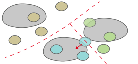
Figure 1060. Virtual borders (red dashed line) dividing the parent-child areas. Arrow indicates to which parent the child belongs. Size of the child intersection with the parent area determines to which parent it belongs.
Produces a table where rows contain children (and their features) with their relevant parents (and their features) and a distance. Specify whether the objects are inside or neighboring the parent (Type) and set their Reference (see Measurement > Object parenting > Child Distance).
This node uses the same settings for Type already described in Measurement > Object parenting > Aggregate Children.
calculates distance between the parent center and the child center.
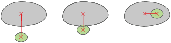
Figure 1061.
calculates distance between the parent center and closest point on the child border.
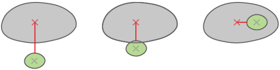
Figure 1062.
calculates distance between the child center and the closest point on parent border.
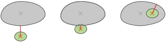
Figure 1063.
calculates distance between the parent border and the child border (minimal distance between borders). When the child touches the parent (middle case), the distance is 0.
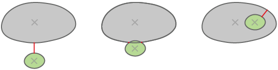
Figure 1064.
The child relationship with its parent is detected using the Child ID action. It adds a “ChildId” feature column (highlighted green) and maps the “ParentId” to “ObjectId” identification column (highlighted red).
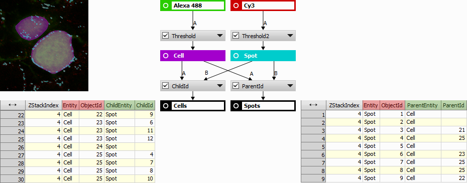
Figure 1065.
Example 14. Simple counting of spots (child) inside cells (parent)
The Child ID action gives the result directly in a natural column order.
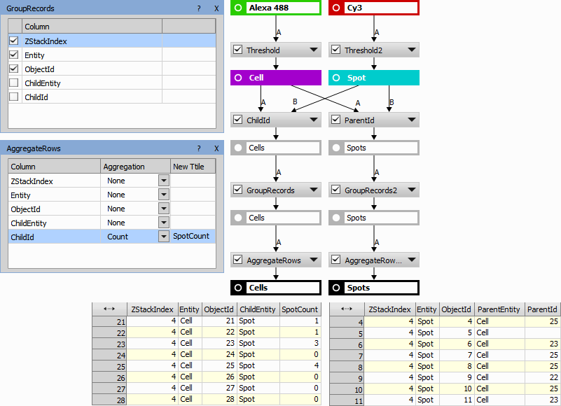
Figure 1066.
Statistics of spot features per cell can be done by adding “SpotFeatures” to “Spots” (from “ParentId”) as they have the same number of rows (all spots) followed by “GroupRecords” and “AggregateRows”.
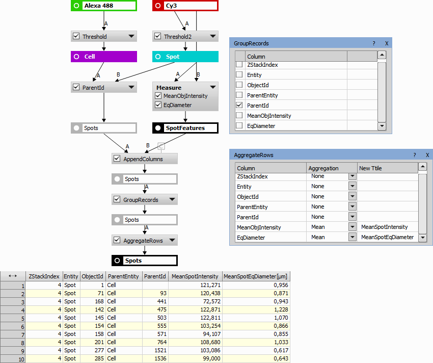
Figure 1067.
Condition
This node uses the same settings for Type already described in Measurement > Object parenting > Aggregate Children.
Calculates distance between parent and child objects. Every parent object can have zero or multiple childs.
This node uses the same settings for Type already described in Measurement > Object parenting > Aggregate Children.
This node uses the same settings for Reference already described in Measurement > Object parenting > Children ![]() .
.
Produces a table where rows contain parents (and their features) with their relevant nearest children (and their features). Specify whether the objects are inside or neighboring the parent (Type) and set their Reference (see Measurement > Object parenting > Child Distance).
This node uses the same settings for Type already described in Measurement > Object parenting > Aggregate Children.
This node uses the same settings for Reference already described in Measurement > Object parenting > Children ![]() .
.
Relationship of the parent with its child is detected using the Parent ID action. It adds a “ParentId” feature column (highlighted green) and maps the “ChildId” to “ObjectId” identification column (highlighted red).
Figure 1068.
Condition
This node uses the same settings for Type already described in Measurement > Object parenting > Aggregate Children.
Calculates distance between child and parent objects. Every child object can have only one or zero parents.
This node uses the same settings for Type already described in Measurement > Object parenting > Aggregate Children.
This node uses the same settings for Reference already described in Measurement > Object parenting > Children ![]() .
.
Shows the X and Y distance from the top left corner to the center of gravity of each object.
Shows the X and Y distance in pixels from the top left corner to the center of gravity of each object.
Shows absolute coordinates of the center of gravity of each object in the scope of the stage XY range.
Shows the X and Y coordinate of the object's centroid in pixels.
Shows absolute coordinates of the centoid of each object in the scope of the stage XY range.
Creates a table with calibrated values of the geodesic centers for all binary objects present in the connected layer. See also Binary processing > Detect > Geodesic Centers.
Creates a table with pixel values of the geodesic centers for all binary objects present in the connected layer. See also Binary processing > Detect > Geodesic Centers.
Please see StartX.
Shows the start coordinates of each object in pixels. Please see StartXpx.
Shows the bounds of each object. Please see BoundsLeft.
Shows the bounds of each object in pixels. Please see BoundsPxLeft.
Shows the absolute bounds of each object. Please see BoundsAbsLeft.
This node thresholds 3D objects.
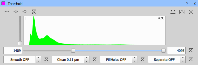
Figure 1069.
 Custom Range
 Zooms to the current range.
 Actual Range
 Zooms to the minimum - maximum range.
 Full Range
 Zooms to the full domain.
These binary processing functions can be activated and their value adjusted using the arrows or directly by typing the value into the edit box. Fill Holes processing can only be turned on/off whereas the values of other processings are applied as a radius in µm or px.
For more information about RGB thresholding please see Thresholding.
This node quickly thresholds 3D objects simply by setting the low and high threshold limit.
For more information about RGB thresholding please see Thresholding.
This command detects bright circular objects within a 3D space. Please see Binary > Spot Detection > Bright Spots for further description.
Note
General analysis 3 spot detection uses the Different Sizes object detection method.
This command detects dark circular objects within a 3D space. Please see Binary > Spot Detection > Dark Spots for further description.
Note
General analysis 3 spot detection uses the Different Sizes object detection method.
![]()
Removes small objects from 3D binary image. See also Binary > Clean  .
.
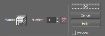
Figure 1070.
![]()
Smooths binary image contours in 3D. See also Binary > Smooth.
Smooths every binary voxel using sphere of the specified radius.
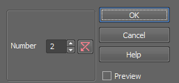
Figure 1071.
Separates binary objects into multiple smaller objects. The higher Count, the fewer objects will separate.
Figure 1072.
![]()
Fills holes inside 3D binary objects present in the current volume. Holes touching image borders are not filled.
![]()
Performs morphological opening on 3D binary image. See also Binary > Open.
Figure 1073.
![]()
Performs morphological closing on 3D binary image. See also Binary > Close.
Figure 1074.
![]()
Performs morphological erosion on 3D binary image. See also Binary > Erode.
Figure 1075.
![]()
Performs morphological dilation on 3D binary image. See also Binary > Dilate.
Figure 1076.
![]()
Removes small holes from 3D binary image. See also Binary > Close Holes.
Figure 1077.
Euclidean Open performs Euclidean Erosion followed by Euclidean Dilation. It clears all areas which cannot contain a circle/sphere of the specified radius.
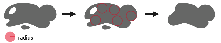
Figure 1078.
See Also
Binary > Open
Euclidean Close performs Euclidean Dilation followed by Euclidean Erosion. It fills all areas of background which cannot contain a circle/sphere of the specified radius.
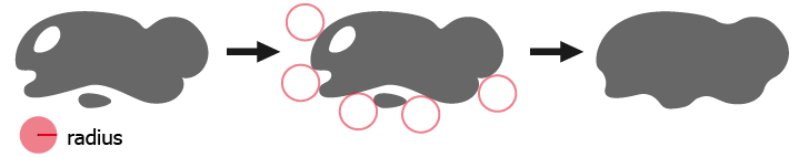
Figure 1079.
See Also
Binary > Close
Euclidean erosion sets each pixel to the value computed as minimum from all pixels within the specified Radius. This will shrink/remove binary objects in the image.
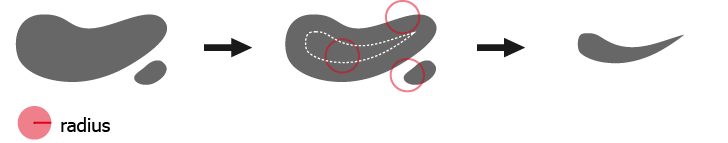
Figure 1080.
See Also
Binary > Erode
Euclidean dilation sets each pixel to the value computed as maximum from all pixels within the specified Radius. This will enlarge/merge binary objects in the image.
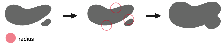
Figure 1081.
See Also
Binary > Linear Morphology > Dilate
Calculates and marks the centroid of the 3D objects found in the connected binary image.
This command calculates and marks the centroid on the 3D binary image. If bright/dark (Signal is) areas dominate aside of the centroid position calculated from just the binary layer, the centroid will be shifted in that direction.
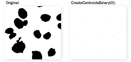
Figure 1082.
For each binary voxel, this function computes its euclidean distance from the nearest voxel of background and displays it as intensity. Output is a floating-point image.
This function expands non-convex 3D binary image objects to their convex boundaries.
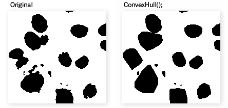
Figure 1083. Example
Creates medial axis from the connected 3D binary objects.
Performs the watershed (flooding) algorithm starting from the connected 3D binary objects. The flooding is based on image pixel intensities.
Defines the direction of flooding - from high intensities (From Bright Regions) or from low intensities (From Dark Regions).
Grows each binary object by a circle (2D) / sphere (3D) of the specified radius. Objects will not be merged together.
Grows each binary object up to the specified intensity. Objects will not be merged together.
will grow from maximum intensity to the specified intensity.
will grow from minimum intensity to specified intensity.
Creates 1pixel seeds out of a skeletonized 3D binary image. This function serves for automatic recognition of the intersection points of single-pixel lines.
Creates 1pixel seeds out of a skeletonized 3D binary image. It preserves only ending points of the skeleton and clears all other pixels.
Selects binary objects from the binary image which are present in input table.
Deletes binary objects from the binary image which are present in input table.
Removes binary objects touching the volume border.
Removes binary objects touching the volume frame. Select Units and the limit values of the frame. Then choose a Mode defining which objects are to be removed.
Please see Binary processing > Colors & Numbers > Color by Id.
Assigns any color to any value of the selected source column used from the connected table.
See also: Binary processing > Colors & Numbers > Color by Value.
Please see Binary processing > Colors & Numbers > Renumber Objects.
Renumberes the binary objects with values taken from the the connected table. Source column has to be specified.
Please see Binary operations > Binary x Binary > And.
Please see Binary operations > Binary x Binary > Or.
Please see Binary operations > Binary x Binary > Xor.
Please see Binary operations > Binary x Binary > Subtract.
Please see Binary operations > Binary x Binary > Equivalence.
Please see Binary operations > Binary x Binary > Having.
Please see Binary operations > Binary x Binary > Not Having.
Please see Binary operations > Single Binary > Invert.
Shows the time and center of the 3D object for tracking.
Shows the time and center of the 3D object for tracking in absolute (stage) coordinates.
Shows the time and the center of gravity of the 3D object for tracking.
Shows the time and the center of gravity of the 3D object for tracking in absolute (stage) coordinates.
Creates a table with all frames and groups them by the track. Enables filtering based on the number of segments (Min segment count).
Creates a table with points of MSD (Mean squared displacement) curve. Select the Track ID, Time and Position columns. Before analyzing using this node use Accumulate Tracks (Tracking > Tracks > Accumulate Tracks) to group by “Track ID”.
Please see example: The NEMO Dots Assembly: Single-Particle Tracking and Analysis.
MSD Curve is generated for each group separately. If you want to have one curve for each track, group the table by Track ID. If you want one curve in total, ungroup the table.
Return CASA motility features.
Specifies the average path velocity parameter.
Calculates derivation of the value in time ((Fi - Fi-1) / (dT)), while requiring Diff Time.
Please see Tracking Output Calculation.
This graph is used for visualizing Y of ordinal X. Settings of each tab are described below.
General
Sets the title of the graph shown in the top.
Sets the inside color of the graph (color behind the visualized data).
Sets the outside color of the graph (frame around the visualized data).
Returns the colors to the default dark scheme.
Sets the color of the axes.
Sets the color of the texts.
Returns the colors to the default light scheme.
Sets the color scheme for the grouped data.
Shows data values directly in the graph.
Hides the legend.
Shows the legend inside the graph. Choose the legend position in the drop-down menu next to this option.
Shows the legend below the graph.
Sets the background color of the legend.
Sets the color of the legend text.
Data
This tab is used to pair the graph axes with the variables available in the table input. Select a data variable and click on the arrow ![]() next to the selected axis to assign it to this axis. Multiple variables can be assigned to the Y axes.
next to the selected axis to assign it to this axis. Multiple variables can be assigned to the Y axes.
 button opens the Data Series dialog setting up the data series graph properties such as the color, line type, stroke type, line width, fill, marker type, and values type. Only the checked properties are visualized in the graph.
 button opens the Error Bar dialog setting up the error bar properties for the selected column. Choose an error column from the drop-down menu and optionally set its color, line width, and whisker width.

 butons move the variable in the axis list up/down.
 button moves the variable from the axis list back to the All Columns list.
X Axis/Y Axis/Left Y Axis/Right Y Axis/Color Axis/Size Axis/Category Axis
Sets the title of the axis that is currently being set.
Reverses the range of the category axis.
Shows/hides the labels for the axis currently being set.
Specifies the axis label format for the axis currently being set.
Specifies the axis label numeral precision.
Specifies the step size of the category axis.
In Auto mode, the minimal value for the range is set automatically. If switched to Fixed, a minimal value from which the data are visualized can be entered into the edit box. Scale specifies the scale type - linear or logarithmic.
In Auto mode, the maximal value for the range is set automatically. If switched to Fixed, a maximal value to which the data are visualized can be entered into the edit box. Reversed Range reverses the values range from “min - max” to “max -min”.
In Auto mode, the major step value for the ticks and gridlines is set automatically. If switched to Fixed, a major step value used for the ticks and gridlines visualization can be entered into the edit box. If Tick is checked, a short tick is added to the axis next to each major step value. Grid color specifies the color of the grid line.
In Auto mode, the minor step value for the ticks and gridlines is set automatically. If switched to Fixed, a minor step value used for the ticks and gridlines visualization can be entered into the edit box. If Tick is checked, a short tick is added to the axis next to each minor step value. Grid color specifies the color of the grid line.
Provides a graphical representation of data where the individual values contained in a two-dimensional matrix are represented as colors from selected color gradient map. This graph does not support grouped source table A.
All tabs are closely described in the Results > Graphs > Barchart node.
Typical Usecases
This graph is used for visualizing Y as function of X.
All tabs are closely described in the Results > Graphs > Barchart node.
This graph is used for visualizing a cloud of points. If the source table A is grouped the graph shows them in colors.
All tabs are closely described in the Results > Graphs > Barchart node.
This 3D graph is used for visualizing a cloud of points. The third axis is visualized using a color gradient. This graph does not support grouped source table A.
All tabs are closely described in the Results > Graphs > Barchart node.
This 3D graph is used for visualizing a cloud of points. The third axis is visualized using disks of different size. This graph does not support grouped source table A.
All tabs are closely described in the Results > Graphs > Barchart node.
Depicts groups of numerical data through their quartiles as a box plot. It shows minimum, first quartile, mean, third quartile and maximum. It can optionally show outliers. If the source table A is grouped the graph shows one box for each group.
All tabs are closely described in the Results > Graphs > Barchart node.
Creates an HTML document with a table input. After setting the parameters and creating the content, click to add the document as a tab to the result table. From there it can be printed (Print), exported to PDF (Print to PDF) or saved as HTML (Save As HTML).
Selected coding format.
Number of connected table inputs.
HTML script area.
The default state serves as an example of formatting the content in Markdown and referencing input tables or their cells.
Code example:
# Markdown Overview

Basic text formatting: *emphasized*, **bold text**, ~strikeout text~.

For details see [Markdown basic syntax](https://www.markdownguide.org/basic-syntax/).

Paragraphs are delimited by *empty* line.
Linebreak are ignored unless there are more spacfes at the end of a line.
Like **here**
where the newline is forced.

HTML code can be used as well:
A<sup>2</sup> + B<sup>2</sup> = C<sup>2</sup>

## GA3 table Inputs

enclose the parameter name into `&` and `;` (`code` is an inline code block)

&T;

or index a specific value (indexing is zero based, first is column second is row):
&T[0,1];

## JavaScript block

JavaScript block may be embedded inside `${` and `}$` with a return statement. During
run whole block is replaced by the returned value. Tables are made available as t, t1, t2, ...

${ return "T[0, 1]<sup>2</sup>: " + Math.pow(t[0][1], 2); }$

## Markdown supports lists

### Ordered lists

1. First item
2. Second item
3. Third item

### Unordered lists

- unordered item
- another one
- third one
- ...

### Nested lists

- unordered item
   - first (starts with three spaces at least)
   - second
- another one
   - first
   - second

## Quoted blocks

> First line
first line continues (more spaces follow)
another line of quote

## Tables

After the header at least three dashes per column are required.

| Value | Name   |
| ----- | ------ |
| 1     | one    |
| 2     | two    |
| 3     | three  |

For details see [Markdown extended syntax](https://www.markdownguide.org/extended-syntax/).

## Color chips

RGB colors: `#FF0000``#00FF00``#0000FF`CSS style area.
Reverts any style changes.
Applies the settings and creates a new tab in the results table.