Data management
Basic

Grouping
Sort & Select
Table Manipulation
Statistics
Statistical tests
Position
Processing
Curve Fitting
Detect
Sequences
JavaScript
frames and objects
cells (objects) and nuclei (objects)
Create a table with the example data and group it by the “group” column.
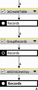
Figure 1018. Analysis definition.
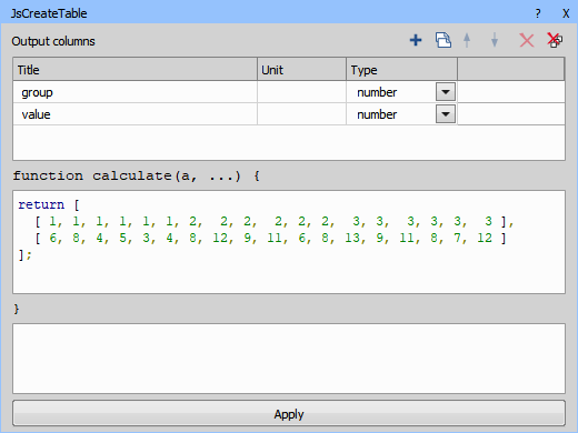
Figure 1019. JS Create Table node.
return [
[ 1, 1, 1, 1, 1, 1, 2, 2, 2, 2, 2, 2, 3, 3, 3, 3, 3, 3 ],
[ 6, 8, 4, 5, 3, 4, 8, 12, 9, 11, 6, 8, 13, 9, 11, 8, 7, 12 ]
];
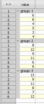
Figure 1020. Grouped data.
Setup the ANOVA and get the results.
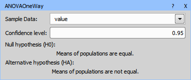
Figure 1021. ANOVA One-way node.

Figure 1022. Results.
the hypothesis that the means of a given set of normally distributed populations, all having the same standard deviation, are equal.
the hypothesis that a proposed regression model fits the data well.
the hypothesis that two normal populations have the same variance.
Please see F-test.
Measurement on the whole image file is performed frame-by-frame (volume-by-volume). Accumulate Records action can be used once or multiple times to obtain records (table rows) from all frames (or volumes) in the selected loop. By default (without accumulate) for performance reasons, records are generated per frame (or per volume). In order to work (sorting, filtering, calculating statistics, ...) on a larger record, use accumulate.
Which loop to accumulate. Select All Loops to process all data at once.
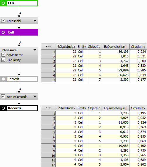
Figure 992. Accumulate Records showing the results when the action is applied (bottom table) and analysis without the action (top table).
Columns from the input tables are appended in the order that they appear. This is useful when joining more features measured on the same number of objects. Number of records across all input tables is expected to be the same.
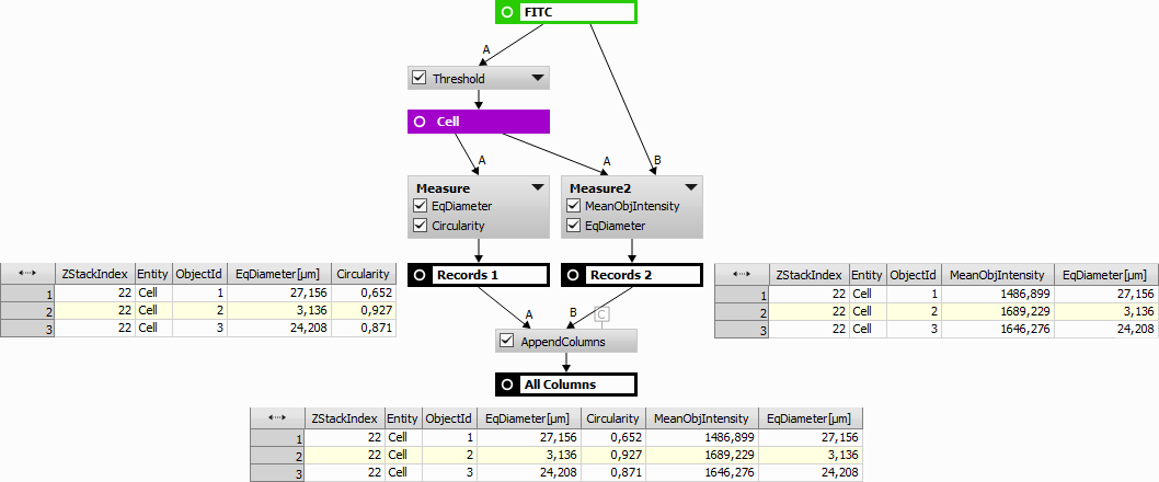
Figure 993. Append Columns action results shown in the bottom table. Left table belongs to “Records 1” whereas the right table belongs to “Records 2”. EqDiameter feature is duplicated.
This node simply works as a calculator with pre-defined operators. Existing columns or their statistics (see Data management > Grouping > Aggregate Rows) can be used as variables. Type of the calculated column and Unit should be set first. Once the calculation is written, confirm it by clicking .
Selects which features are displayed in the resulting table, change their order using the arrows, change their name (New Title), number format (New Format) and Precision.
Note
The Modify Table Columns dialog having the same functionality as this node can be opened directly from Analysis Results by clicking  .
.
Groups records and computes the selected statistic of rows. If the table is grouped the statistic is calculated for each group. Each group of rows becomes one row in the output table.
For more information about grouping see Data management > Grouping > Group Records, for more information about statistics see Data management > Grouping > Aggregate Rows.
This node is used for changing units, skipping values and similar tasks. Select the Column which is about to be changed, define the new Unit (NewVal example is shown below) and set the value Offset or Gain. No new column is created, only the values in the source column are skipped.
Aggregate Rows computes the selected statistic of rows. If the table is grouped the statistic is calculated for each group. Each group of rows becomes one row in the output table.
Table 6. Aggregation Statistics
| None | Any value (typically first). |
| Total | Number of values including empty (null). |
| Count | Number of values not including empty (nulls).* |
| Distinct | Number of distinct (unique) values. |
| Mean | Mean value. SUM(values)/N.* |
| Median | Middle value of all ordered values.* |
| Sum | All values added.* |
| Min | Minimum value.* |
| Max | Maximum value.* |
| StDev.P | Population Standard deviation.* |
| StDev.S | Sample Standard deviation.* |
| Var.P | Population Variance.* |
| Var.S | Sample Variance.* |
| VarCoef.P | Population Coefficient of Variation.* |
| VarCoef.S | Sample Coefficient of Variation.* |
| StErr.P | Population Standard Error.* |
| StErr.S | Sample Standard Error.* |
| Skewness.P | Population Skewness.* |
| Skewness.S | Sample Skewness.* |
| Kurtosis.P | Population Kurtosis.* |
| Kurtosis.S | Sample Kurtosis.* |
| RootMeanSquare.P | Population Root Mean Square.* |
| RootMeanSquare.S | Sample Root Mean Square.* |
| Coalesce | First not empty (non-null) value. |
| LastMinusFirst | Last value minus first (values[N-1] - values[0]) |
| First | First value (values[0]) |
| Last | Last value. (values[N-1]) |
| Mode | Mode.* |
| Entropy | Entropy.* |
| HistoUniformity | Uniformity of histogram (link to Measurement - Uniformity).* |
| QuartileQ1 | First Quartile.* |
| QuartileQ3 | Third Quartile.* |
| PercentileP01 | 1st Percentile.* |
| PercentileP05 | 5th Percentile.* |
| PercentileP10 | 10th Percentile.* |
| PercentileP90 | 90th Percentile.* |
| PercentileP95 | 95th Percentile.* |
| PercentileP99 | 99th Percentile.* |
* Does not include empty (null) values.
Filters whole groups (selected in the Column) based on the selected Statistics per group. Define the filtering using the Comparator drop-down menu and the Value edit box.
This node uses aggregation statistics. Please see Data management > Grouping > Aggregate Rows.
All rows are in one group by default. Rows having an equal given column (selected in the Group Records action) form a group which is visualized in the table. Grouping is used with statistics (Aggregate Rows) for calculating per group (BinaryLayer, ZStack, Object...) aggregates. Only limitation is that the result of the grouping is currently not visible in the preview and in the final result.
Previously grouped records are ungrouped by this action.
Filters records associated to the current frame. This node is useful only when the connected table is accumulated.
This action can be used to filter table records (rows) using a selected column. Resulting table contains only the rows satisfying the filter condition applied to the given column.
Column to be filtered.
Comparison operator.
Comparison operand.
Example 12. Filter Records action used in series to act as an intersection. Both conditions (10 <= EqDiameter AND 0.9 <= Circularity) must be met at the same time.
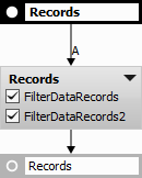
Figure 995.
Example 13. Filter Records action used in parallel to act as an union. One or both conditions (10 <= EqDiameter OR 0.9 <= Circularity) must be true.
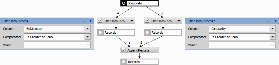
Figure 996.
This node “pivots” the input table by the specified Pivot Column (“ObjectId” in the example below), thus it creates a new column for each “ObjectId” value. The new column will contain values of columns having a column Role in the bottom definition table (“Entity” and “EqDiameter” in the example below). E.g. in the second column of the results table, the “EqDiameter” values for objects with ID==1 are arranged in rows by the “ZStackIndex”. The number of rows depends on the possible combinations of all values of columns marked with the role Row. Each column will be present for the first number of values specified in the Column Count edit box. The order of the columns is specified by the Column Order switch. In our example below, Append would add 10x Entity whereas Mix orders them: Entity, EqDia, Entity, EqDia, etc. Column Suffix sets the name of the created column. PIVOT_NAME (“ObjectId” in our example) and PIVOT_VALUE (“ObjectId” value) or any other text can be used here.
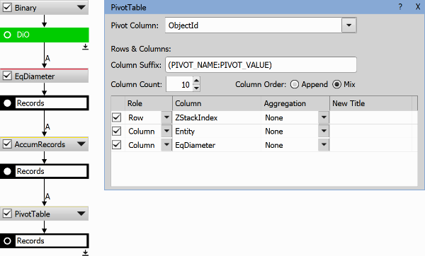
Figure 997. Pivot Table example
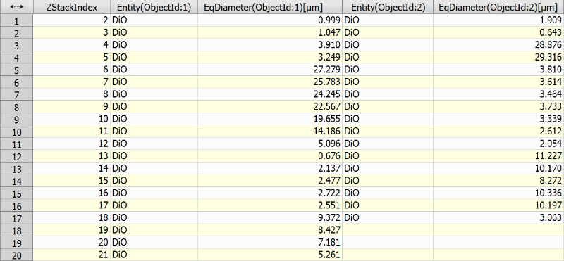
Figure 998. Pivot Table example results
Shows the first and last record from the connected table.
Select Records action takes a specified number of records (Count) from a selected starting row (First Row). Typical use-case is to select the first row of a sorted record set.
Reorders the records based on a given column and then shows the defined number of records (either smallest or biggest). This node is a combination of Sort Records, Reverse Records and Select Records.
Sort action reorders records so that the selected column is sorted in an ascending order.
Appends records (rows) from input tables one by one into the output table. If an input table contains a column already present (has same column ID) in the output table (from the preceeding input tables) it will use it (i.e. not append a new column).
The resulting table is ordered by the identification columns.
Every column has an implicit ID (invisible to the user) given to it by the node that creates the column. The ID is used internally to reference columns. Therefore, even after a column is renamed it is still correctly pointed to by subsequent nodes. Consequently, columns are considered “same” if they have the same ID. Special identification columns like Loop indexes, Object Entity, Object IDs are given the same ID for each special column. Therefore ObjectID column will be considered the same from all tables. This behavior is usually expected. If not, it can be altered with these nodes: Data management > Table Manipulation > Copy Column ID, Data management > Table Manipulation > New Column ID and Data management > Table Manipulation > Compact Columns.
Appending records is useful when joining two tables with the same columns. For example for joining two disjunct filtrations or aggregations.
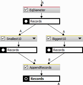
Figure 999.
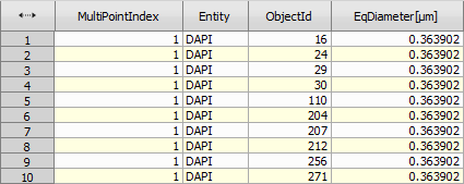
Figure 1000.
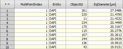
Figure 1001.
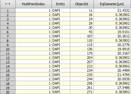
Figure 1002.
Aggregates all columns with the same title (or title different just in numerical suffix) to the first column using the First Valid rule.
This is useful when Data management > Table Manipulation > Join Records or Data management > Table Manipulation > Append Records produces duplicate colums because of their different IDs (please see Data management > Table Manipulation > Append Records for more on Column IDs).
For more control on which columns will merge use Copy Column ID.
The following example demonstrates how to force two different columns to merge into single one using Data management > Table Manipulation > Append Records.
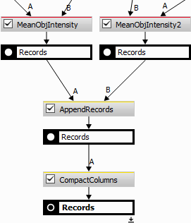
Figure 1003.
After append records there are two columns MeanObjectIntensity and MeanObjectIntensity2 that need to be merged into one.
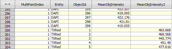
Figure 1004.
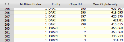
Figure 1005.
The resulting table contains all columns from table A with specified columns IDs replaced with IDs from reference table B.
This is useful when tables A and B are intended to be merged using Data management > Table Manipulation > Join Records or Data management > Table Manipulation > Append Records node and they contain columns with different IDs (please see Data management > Table Manipulation > Append Records for more on Column IDs) that should be treated as same column.
There is a simpler automatic way using Data management > Table Manipulation > Compact Columns.
The following example demonstrates how to force two different columns to merge into a single one using Data management > Table Manipulation > Append Records.
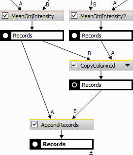
Figure 1006.
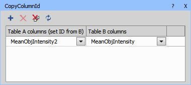
Figure 1007.
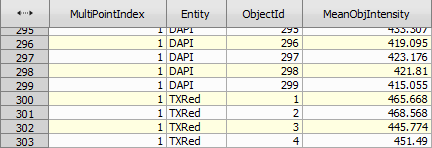
Figure 1008.
This action is useful for merging incompatible tables:
It joins records from two or more unrelated (with different number of rows and columns) record sets. Resulting table contains a union of all distinct input table columns (loop indexes, entity and Object Ids are considered the same).
Select the type of join (see below) and click  to add a table row where you specify the relation between the joined features taken from two different tables.
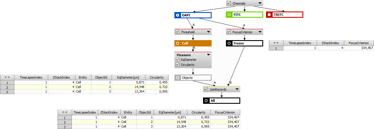
Figure 1009. Join Records action results shown in the bottom table. Left table belongs to “Objects” whereas the right table belongs to “Frame”.
Inner Join outputs a Cartesian product of the related rows (rows where “using columns” have same value):
CountRows(R) = CountRows(A) × CountRows(B) × CountRows(C) × ...,
where A, B, C, ... are input tables and R is an output table.
A related row (e.g. ZStackIndex = 3) must be present in all tables.
Left Join is an inner join plus all related rows which do not occur in tables to the right. All rows from the leftmost table (A) are in the result table (R).
Right Join is the same as the Left Join but with reversed input cables (... C, B, A).
Makes the specified columns IDs unique (please see Data management > Table Manipulation > Append Records for more on Column IDs).
It is useful when nodes like Data management > Basic > Append Columns, Data management > Table Manipulation > Join Records and others treat a column coming from two different tables as the same one and does not include it twice. This is typically because both columns were made by one node or the is a “system” column like Loop Index Columns, Entity or Object ID.
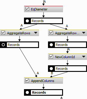
Figure 1010.

Figure 1011.

Figure 1012.

Figure 1013.
Without the Data management > Table Manipulation > New Column ID node both source columns are merged (overwritten) into one.

Figure 1014.
Shifts data in selected columns by given number of rows.
Fill
Rows which are empty after shift are left empty.
Rows which are empty after shift are filled with original values.
Rows which are empty after shift are filled with values of rows on the other end of columns.
Aggregate Columns action creates a new column with the given name (Title) in which the result of a calculation is placed (Aggregation). The calculation is based on the checked parameters.
Name of the new column.
Statistics to be computed.
Checked columns will be used for calculation.
This node uses aggregation statistics. Please see Data management > Grouping > Aggregate Rows.
Creates new bin column and assigns each row to one bin based on the value of the selected column. Then the rows can be grouped based on the bins.
Column for binning.
Name of the new bin column.
Sets the column type either to a Number or a String (sequence of characters).
Unit of the new bin column.
 Add bin
 Adds a new table row (one bin).
 Remove selected bin
 Deletes a row record (one bin).
 Remove all bins
 Clears the table (deletes all bins).
Generate bins automatically Opens the Generate Bins window used to calculates linear or logarithmic bins based on the bin width. Set the lower starting value of the bin set (Min), then the higher ending value (max) and enter the width of the bin. Choose whether the generated bins will be Linear or Logarithmic with a specified base. Set the Label for each newly generated bin. Enter “lo” to start from the lowest generated value or “hi” to start from the lowest generated value + width. Any other mathematical combination of “lo” and “hi” is also possible (see the examples below).
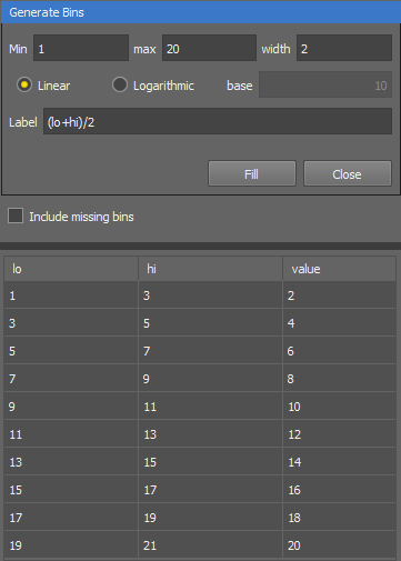
Figure 1015. Linear method generating the middle value of each bin.
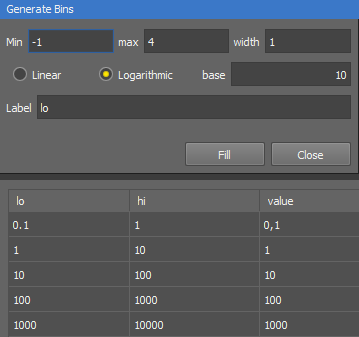
Figure 1016. Logarithmic method generating logarithmic bins to base 10.
 Validate bins
 If the bins are created improperly, this function automatically corrects the classes so that they follow each other.
 Copy to clipboard
 Copies the full table to clipboard.
 Paste from clipboard
 Inserts the table data from clipboard into the frequency table.
Fill in the table so that lo and hi values represent the bin size and value sets the user defined label to each bin. When lo or hi is empty (null), it is interpreted as negative infinity or positive infinity respectively. Bins should be exclusive otherwise the behavior is not defined.
Creates a new column and fills it with bin labels to which the value in the source column falls into. Bins are equidistant intervals between min and max.
Name of the new column.
Column for binning.
Minimal bin value.
Maximal bin value.
Number of bins.
Sets options how each bin is labeled (Start point: min of each bin, Middle point: middle of each bin, Bin class Id: bin index starting from 1.
This table can be used to classify the results data to see the number of elements in each defined class. Select the Source column, name the New column and add units (Unit). Fill in the table so that From and To values represent the bin size (range of source values) which will be substituted by the new value specified in the third column.
Other tools are similar to the Data management > Statistics > Binning node.
(requires: Local Option)
Creates a table with points of Probability density function or Cumulative distribution function. Select Distribution, its Parameters, interval Endpoints and Step. If checked, y- values of Critical Region are generated to separate column. Tested Value is generated to separated column as well.
Creates a summary statistics table, as seen in the example below.
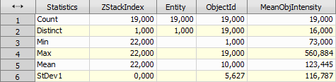
Figure 1017.
This node uses aggregation statistics. Please see Data management > Grouping > Aggregate Rows.
(requires: Local Option)
Performs One-way ANOVA (analysis of variance). Please see one-way ANOVA.
Select a column with Samples Data and parameters of the test. The table must be grouped. Every group is one factor (i.e. treatment group). The output results of the analysis are displayed in a one row table.
Working example from a Wikipedia page:
(requires: Local Option)
This test can be used to test:
Select Sample A from table A, Sample B from table B and parameters of test. If tables are grouped, then count of the groups in each table must be same. F-test is done for each pair of the groups (i-th group in table A and i-th group in table B). Output is a table with one row of data for each group pair.
(requires: Local Option)
This is a location test of whether the mean of a population has a value specified in a null hypothesis (please see t-test).
Select Sample and parameters of test. If table is grouped, then the t-test is done for each group. Output is a table with one row of data for each group.
(requires: Local Option)
Paired samples t-tests typically consist of a sample of matched pairs of similar units, or one group of units that has been tested twice (a "repeated measures" t-test). A typical example of the repeated measures t-test would be where subjects are tested prior to a treatment, say for high blood pressure, and the same subjects are tested again after treatment with a blood-pressure-lowering medication. By comparing the same patient's numbers before and after treatment, we are effectively using each patient as their own control (please see t-test).
Select Sample A, Sample B and parameters of test. If table is grouped, then the t-test is done for each group. Output is a table with one row of data for each group.
(requires: Local Option)
The independent (unpaired) samples t-test is used when two separate sets of independent and identically distributed samples are obtained, one from each of the two populations being compared. For example, suppose we are evaluating the effect of a medical treatment, and we enroll 100 subjects into our study, then randomly assign 50 subjects to the treatment group and 50 subjects to the control group. In this case, we have two independent samples and would use the unpaired form of the t-test (please see t-test).
Select Sample A from table A, Sample B from table B and parameters of test. If tables are grouped, then count of the groups in each table must be the same. t-test is done for each pair of groups (i-th group in table A and i-th group in table B). Output is a table with one row of data for each group pair.
Calculates Z-factor for positive and negative control groups.
Select column containing labels (positive, negative and others).
Select column containing measured control values.
Enter label of rows with negative control (in Labels column).
Enter label of rows with positive control (in Labels column).
Check to create column with Z-factor value and enter its name.
Vectorally adds two positions. Z positions are optional. The result is two or three new columns (X, Y, (Z)).
ResX = X0 + X1, ...
Vectorally subtracts two positions in time. Z positions are optional. The result is two or three new columns (X, Y, (Z)).
ResX = X0 - X1, ...
Calculates the distance between two points in time. Z positions are optional. The result is two or three new columns (X, Y, (Z)).
Dist = SQRT( (X0 - X1)^2 + (Y0 - Y1)^2 + (Z0 - Z1)^2 )
Calculates the length of the vector. If Z (Vector Z) column is left blank 2D length is calculated:
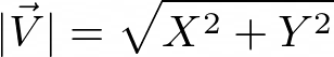
Figure 1023. Vector Length in 2D
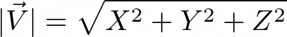
Figure 1024. Vector Length in 3D
Calculates the heading of the vector. Heading is the angle in degrees between the positive X axis and the  counterclockwise in range <0; 360>. Elevation is calculated as well when the Z (Vector Z) column is given. Elevation is the angle in degrees between the XY plane and the in range <-90; 90>.
Transforms (recalculates) the position coordinates between the stage (absolute) and the image (relative) system.
Defines the X, Y, Z positions.
Defines the source and destination format of the position.
Name of the transformed features.
Unit of the transformed features.
Only the local extreme values found in the source Column are copied into the new column. Name the New Column and specify its units (Unit). Select which Extrema are taken into account and adjust the Threshold to filter out subtle changes.
Calculates the rolling average value as an average of three consecutive values (current value and the value before and after the current one). Select the Column from which the rolling average will be calculated, name the New Column and specify its units (Unit). Use Window Radius to expand the number of consecutive values from which the average is calculated.
Calculates the rolling median value as a median of three consecutive values (current value and the value before and after the current one).
Calculates the rolling minimum value as a minimum of three consecutive values (current value and the value before and after the current one).
Calculates the rolling maximum value as a maximum of three consecutive values (current value and the value before and after the current one).
Fits a curve to data using the method of least squares. Fit values are placed into a new column. Select the Dependent Column and Independent Column, choose the Curve type and specify the Outputs.
Data
Column with independent data, [x]
column with dependent data, [y=f(x)]
Model
Type of the curve in case of higher polynomial curve its degree n.
Table 7. Curve type
| Curve | Formula | Parameters |
|---|---|---|
| Mean | 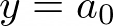 | a0 |
| Linear | 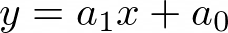 | a1, a0 |
| Quadratic | 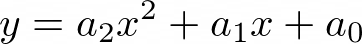 | a2, a1, a0 |
| Higher Polynomial | 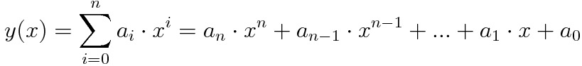 | an, ... , a2, a1, a0 |
| Simple Exponential | 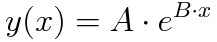 | A, B |
| Gaussian | 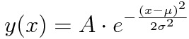 | A, µ, σ |
Note
Gaussian curve is calculated using weighted linear least squares, if it cannot be calculated this way, nonlinear least square method is used instead and  is 0.
is 0.
P-value is often between 0 and 1, higher value shows that parameter is less significant. You can filter out all values higher than given value. This is done iteratively until all p-values are lower than given value.
Outputs
Approximated value given by the resulting equation.
Resulting equation which can be used in a linechart.
Displays goodness of fit, between 0 and 1, higher means better.
Appends columns with parameters.
Appends columns with p-values.
Fits a Dose-Response curve to data using the method of non-linear least squares. Fitted values are placed into a new column.
Data
Column with independent data, [x] i.e. Dose.
Column with dependent data, [y=f(x)] i.e. Response.
Model
Type of the curve in case of higher polynomial curve its degree n.
Table 8. Curve type
| Curve | Formula | Parameters |
|---|---|---|
| 4PL (Symmetrical) | 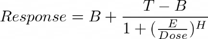 | B, T, E, H |
| 5PL (Asymmetrical) | 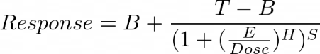 | B, T, E, H, S |
Note
You can constrain (fix) any of the parameters.
Table 9.
| Parameter | Meaning |
|---|---|
| B | Bottom (minimum of the function). |
| T | Top (maximum of the function). |
| E | Inflection point of the curve. |
| H | Hill (hill coefficient), gives direction and how steep the response curve is. |
| S | Gives assymetry around the inflection point. |
EC50, IC50, LD50, ... are same as E for the 4LP model, for 5PL they are calculated as follows:
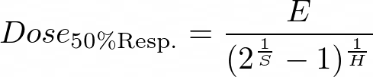
Figure 1025.
Outputs
Approximated value given by the resulting equation.
Resulting equation, can be used in a linechart.
Appends columns with parameters.
Fits multiple gaussian curves to data using the method of nonlinear least squares.
Data
Column with independent data, [x].
Column with dependent data, [y=f(x)].
Model
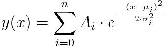
Outputs
Approximated value given by the resulting equation.
Resulting equation containing all curves, can be used in a linechart.
Appends column for each fitted curve.
Appends columns with parameters.
This Density-Based Spatial Clustering of Applications with Noise (DBSCAN) action clusters 2D points. Cluster IDs are inserted into a new column. Name the new column (New Column Name), select the Position X Column and Position Y Column, set the Maximal Distance in Cluster and the Minimal Number of Neighbours. Two points are neighbors if their distance from each other is not greater than the Maximal Distance in Cluster. If any point has at least Minimal Number of Neighbours, this point and all his neighbors are added to the same cluster. If any point is part of a cluster, all of his neighbors are also part of this cluster.
For details about this action, please see the DBSCAN method.
Detects a square grid and appends rows with coordinates of the missing points. Select columns containing coordinates of the grid points and select what to ignore during the detecting of the missing points.
Inserts a new column containing new indexes of binary objects of detected TMA (Tissue microarray) cores. Enter the New Column Name, select the Position X Column and Position Y Column with position of core centers. If you check Skip Gaps, the indexing will not include numbers of missing cores (binaries will be numbered from 1 to N, where N is count of binary objects).
This node automatically detects columns and rows of grid of TMA cores. Then it assigns new indexes so that cores in the upper row have smaller indexes than cores in the lower row. In each row, cores are indexed from left to right. Numbers of missing cores are not used (for example, if you have 10 cores in a 4x3 grid, core in the bottom right corner (if not missing) will always have an index of 12).
For good results cores should be laying in a square grid which is not rotated.
Note
This node can be used on any binary objects laying in a square grid (not just TMA cores).
(requires: Local Option)
Detects run of the same values and returns the column with IDs. Same ID indicates the same values in the Column for subsequent indexes in the Index Column.
Calculates a new column as a difference (subtraction) between the second and first value, third and second, etc. Select the Column from which the difference will be calculated, name the New Column and specify its units (Unit). First record is blank when First item Is Empty is selected.
Calculates a new column as a sum of the first and the second value, second and the third value, etc. First row stays the same. Select the Column from which the integration will be calculated, name the New Column and specify its units (Unit). Enter a Constant if you want to add a number to each sum of the two values.
Computes difference (vector) X, Y, Z columns in every two consecutive rows.

Figure 1026.
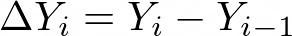
Figure 1027.
Figure 1028.
Adds up X, Y, Z columns in every two consecutive rows.

Figure 1029.
Figure 1030.

Figure 1031.
Figure 1032. Alpha calculation
ΔT is a time interval [s] and fc is a cut-off frequency [Hz].
Please see High Pass Filter for more details.
Figure 1033. Alpha calculation
ΔT is a time interval [s] and fc is a cut-off frequency [Hz].
Please see Low Pass Filter for more details.
Generates a new column with an integer sequence. Name the New Column and set the Start and Step value of the sequence. Optionally the sequence can respect a selected loop over column value if switched from the default <rows> value.
Generates a new column with an exponential sequence. Name the New Column and set the Start and Factor (exponent) value of the sequence. To create an inverted exponential sequence, click and the Factor value is automatically changed. Optionally the sequence can respect a selected loop over column value if switched from the default <rows> value.
Transforms the source record set into the resulting record set that has a new column. The transformation is to be programmed in JavaScript.
See the dedicated documentation: Extending GA3.
Transforms N source record sets into resulting single record set. The transformation is to be programmed in JavaScript.
See the dedicated documentation: Extending GA3.