
General Analysis 3 (GA3) is a versatile instrument designed to construct image analysis procedures in a modular manner. These procedures, here referred to as “recipes”, are created in the GA3 Editor ( View > Analysis Controls > GA3 Editor
  ) and organized through the Analysis Explorer (Analysis Explorer). A GA3 recipe contains a series of actions, such as denoising or thresholding, executed on specific inputs like image color channels or binary layers, ultimately generating the desired outcome. The recipe is graphically represented as an oriented graph, providing a visual representation of the analysis workflow process.
Note
Please refer to the NIS-Express online help for the most up-to-date information, as General Analysis 3 functionality remains identical within NIS-Elements.
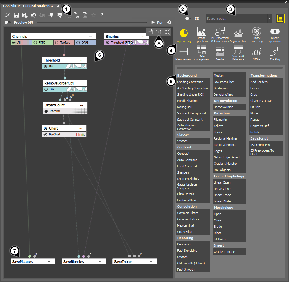
Figure 658. GA3 Editor
Main toolbar
3D nodes switch
Search box
Categories
Groups with nodes
Graph area
Saving nodes
Comments/zooming toolbar
Nodes are arranged within categories and groups, and they can be moved into the Graph area and connected in a sequential manner to form a analysis recipe. The nodes and their links determine the sequence in which they are executed. By connecting the nodes, the output of one node becomes the input for the next node in the chain. The graph consists of action nodes that produce specific intermediate results. Each step within the chain, which influences the final result, can be previewed or modified in real-time.
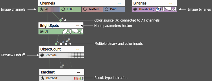
Figure 659. Node anatomy
Preprocessing
Preprocessing aims at improving the image properties for further analysis. The possibilities range from simple nodes such as smoothing or sharpening to complex constructs that create new artificial channels. The relevant nodes are in
 Image Processing),
  Image Operations and
  ND Processing & Conversions categories.
Segmentation
It aims at detecting segments of pixels in the image such as particles, cells, organoids, animals or just foreground in order to be further measured, counted and analyzed. Notable nodes are Threshold and Spot detections in the
 Segmentation category.
Binary postprocessing
The goal of postprocessing is to improve the quality of segmented objects so that they better represent the underlying structures. Typical nodes like cleaning, smoothing or separating are in
 Binary processing and operations such as intersection, union or subtraction are in
  Binary operations.
Measurement
It measures selected features on fields or objects and outputs it in a tabular form. The nodes are in the
 Measurement category.
Data manipulation
The nodes in the
 Data manipulation category work on tables. Typical manipulation include grouping, filtering, joining and aggregating tables. There are also several statistical nodes to calculate simple moments such as mean or standard deviation to more advanced ones like fitting.
Presentation
The aim of presentation nodes is to visualize the data either by plotting graphs like histograms or scatter-plots. It is also possible to display multiple panes to show more tables and graphs simultaneously and in a synchronized way using one of Layout nodes.
bits per channel: 8, 10, 12, 14, 16 bits unsigned integer or 32 bit float image
calibration: microns per pixel
size: width, height
ID: column identifier
Title: what is displayed in the column header.
Unit: displayed in [a.u.]
Type: such as Number or text
Display: number of decimal digits and notation
formulae as a result of fits,
jpeg or png images as thumbnails.
Number
Text
Table
the output of ND Processing & Conversions > Stack reduction > Median contains static part of scene which can be subtracted (Image Operations > Arithmetics > Subtract) from each frame. This is be helpful for segmentation when detecting moving objects.
variance over time-lapse is not built in, but can be constructed (as any higher moment) using built-in nodes using the formula: \(Var(X) = E[(X - E(X))^2]\) where \(E(X)\) can be replaced with the ND Processing & Conversions > Stack reduction > Average node.
Image Operations > Arithmetics > Subtract previous frame from the current with ND Processing & Conversions > Stack reduction > Select Frame.
Threshold on DAPI produces Nuc binary layer with segmented nuclei.
Segmentation > Spot detections > Bright Spots on Alexa 488 produces Spots binary layer.
There are hundreds of nodes that can be used in a recipe. However, there are only few that are used regularly. Others are used sparingly because of their niche role. The nodes are organized into categories and groups in the order as they are typically used.
In the end, it is the use case (image data and the scientific question) that determines which nodes are used and how complex the recipe needs to be.
Some workflows do only image processing (denoising, deconvolution, EDF, …) where the input is an image with some defects and the output is a better image.
Typically the workflow is more complex and involves more steps:
Nodes are listed in groups which are organized in categories. Click on one of the category icons and browse through the node list below or use the search box to find the exact node. When working with 3D binaries, turn the 3D node switch on to automatically update the node list with the 3D nodes.
Multiple instances of each node can be dragged and dropped into the graph area. Each node needs to be connected to its appropriate source, for example:
There are three distinct types of nodes available:
Image intensity (or sometimes called color) data are represented by channels. Channels have real meaning especially in fluorescence imaging where their intensity values are directly proportional to the concentration of the given fluorophore.
There is also another special channel called All or RGB in case of RGB images. RGB and All are treated the same by most nodes. There are, however some nodes that require specifically RGB image. Processing nodes by default process all channels the same. Deconvolution node is the notable exception which allows defining per-channel settings.
The channels parameters have metadata which are assigned before the run of GA3 (during the design of the recipe).
Notably:
All channels must have the same metadata when saved to the ND2 file. They are coerced to maximum value in the save node.
Note
As metadata must be set before the run of GA3 some Control parameters setting the metadata cannot be used as dynamic parameters.
Binaries (a.k.a Binary layers) are typically a result of segmentation. They are made of contiguous patches or segments of pixels representing entities such as cells, spots or organoids. The are displayed as semi-transparent overlays or contours on the image.
The same principles apply to 3D where objects are made of contiguous 3D patches of voxels.
Binary objects may have an ID which links them to the measured features stored in tables. In such case the binary is stored as an “image” of 32-bit integers, where every pixel is a natural number (object ID) or zero (background).
In many situations the object ID is not needed and as it is expensive to compute its pixels are simply marked as objects or background. Stored as 8-bit unsigned integer where zero is the background and non-zero is the object. These objects have implicit IDs going from top-left to bottom-right from 1 to N.
An object to be must not touch others (to be separate objects). It must be divided by one pixel horizontally and vertically.
Binaries have the same limitations as channels regarding metadata during the GA3 run.
Note
Any binary operation or processing nearly always changes the ID of an object. Binary processing > Colors & Numbers > Renumber Objects reassigns IDs to match a previous numbering.
Object numbers in subsequent frames do not match. Use Tracking to match subsequent objects in time.
Tables 2D arrays of values organized into columns and rows. They are the primary result of Measurement.
Columns in GA3 are typically made of one or more book-keeping (called system) columns such as loopIndex for every loop (time, z-stack, multi-point), object ID and entity for objects followed by feature columns.
Book-keeping columns are used to link a table row to frame, volume or object. If a table does not have such columns it looses capability to link to the image data.
Columns have metadata such as:
Book-keeping columns have always the same ID. Other columns have their column ID kept from the moment of their creation. The benefit being that changing the title does not break the downstream nodes (such as graphs) which reference the columns by ID and update with the title change.
When merging tables however, columns may be discarded because of their ID which is same coming from two or more tables where only the leftmost is taken. In such situation use the Data manipulation > Table Manipulation > New Column ID node.
Note
Columns and their metadata are defined before the GA3 runs (same as channel metadata) and cannot be modified during the run.
Rows are filled during the GA3 run. By default tables are processed frame-by-frame or volume-by-volume unless accumulated.
Rows values may contain various data encoded into text such as
Nodes are setup using settings dialogs. Each node have a different more less complex depending of its functionality. Some nodes do not have settings dialog at all.
The set of Control parameters represent the state of the node.
The widgets in the dialog correspond to Control parameters which are:
With a special dialog some Control parameters can turn into input parameters making them “dynamic”.
This is useful when a control parameter (typically a number) has to be set by a preceding node. As an example threshold may take the low limit from minimum intensity or a quantile.
GA3 handles multiple dimensions (ND) like Z-Stack, Time-lapse or Multi-point implicitly. By default it processes the input ND image frame-by-frame in the same order as the frames are stored in the file. The nodes in the graph, may change this behavior. For example 3D nodes switch the processing to volume-by-volume.
Some nodes like the Maximum Intensity Projection (ND Processing & Conversions > Stack reduction > Max IP) or Data manipulation > Basic > Accumulate Records may reduce or completely collapse a dimension. In that case the following nodes operate only on the reduced dimension.
When collapsed outputs are connected into a node together with non-reduced output the former is silently broadcasted back to have the same number of frames as the latter.
For example: ND Processing & Conversions > Stack reduction > Average node when applied to the time-lapse will produce only one frame image containing only the static parts. It can be subtracted from all frames. The Image Operations > Arithmetics > Subtract node will treat the single frame coming from the ND Processing & Conversions > Stack reduction > Average node as if there were as many as in the whole time-lapse.
Here there are some commonly used GA3 graph building patterns.
The Image processing graphs typically connect one (or more) processing nodes one after the other from the source Channels node through All channels and save the result.
Three examples below show three common processing nodes:
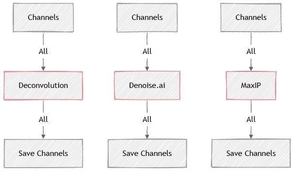
Figure 660.
In many cases it is practical to calculate a projection or Reduction over all a loop and the subtract it from every frame.
In the examples below:
Note
The Subtract broadcasts the single frame input from the Median back to N.
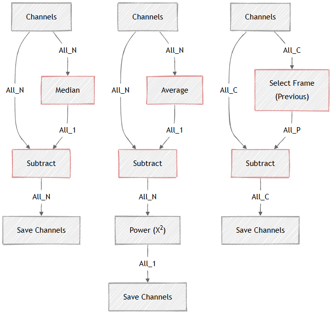
Figure 661.
Segmentation-only graphs create a Binary layer over the original image. Therefore the graphs typically save the original All channels and the binaries from the segmentation.
In the example below two Channels are segmented:
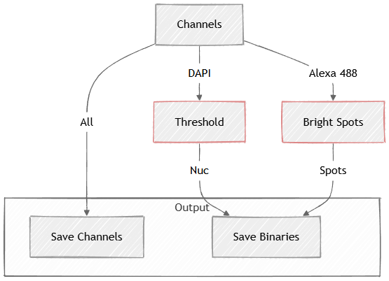
Figure 662.
It measures field features such as channel intensity or ratio of channels. The measurement produces a table with one row per field (typically frame).
Table 13.
| Time [s] | MeanOfDAPI | MeanOfFITC | MaxOfDAPI | MaxOfFITC | MinOfDAPI | MinOfFITC |
| 2.55908 | 304.988 | 210.585 | 3,459 | 4,095 | 0 | 0 |
In the example below there is a Measure field (Measurement > Basic > Field) that has an optional mask input such as ROI that is drawn interactively when the graph is ran.
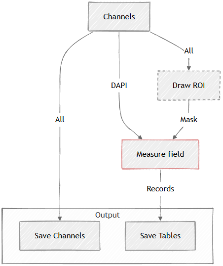
Figure 663.
It measures object features such as size, shape, position or channel intensity. The measurement produces a table with one row per object. The main input of this measurement node is a binary layer and an optional channel for intensity measurement under the binary.
Table 14.
| ObjectId | Area [µm²] | Perimeter [µm] | Circularity | Elongation | MeanIntensity |
| 1 | 23.276 | 21.631 | 0.625 | 2.291 | 14.232 |
| 2 | 4.820 | 12.939 | 0.362 | 6.251 | 20.102 |
| 3 | 9.165 | 12.042 | 0.794 | 1.584 | 26.680 |
| 4 | 16.886 | 16.077 | 0.821 | 1.343 | 10.551 |
In the example below the Measurement > Basic > Object is connected the Obj binary coming from the Threshold and to the All channels for intensity measurement. The original channels, thresholded binaries and the object table are all saved.
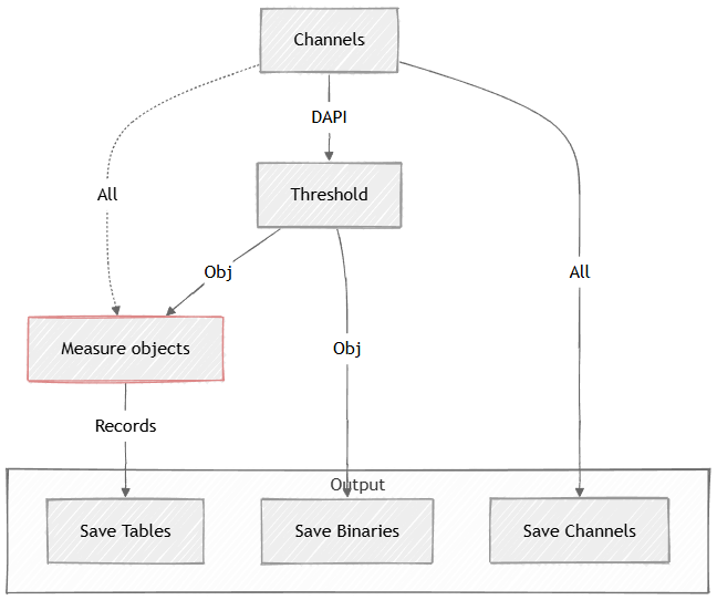
Figure 664.
In many cases where cells must be segmented it is practical to segment nuclei first (as it is easier) and grow them following intensity (using the watershed algorithm) until background intensity is met or another cell is encountered. This technique ensures a relatively correct number of cells with more or less adequate cell shape.
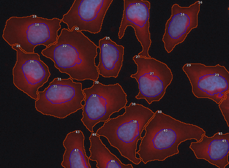
Figure 665.
Then, to ensure that all cells are well-formed (i.e. each has one nucleus and non-empty cytoplasm) use the Binary processing > Cell Processing > Make Cell node before Measurement > Basic > Cell measurement.
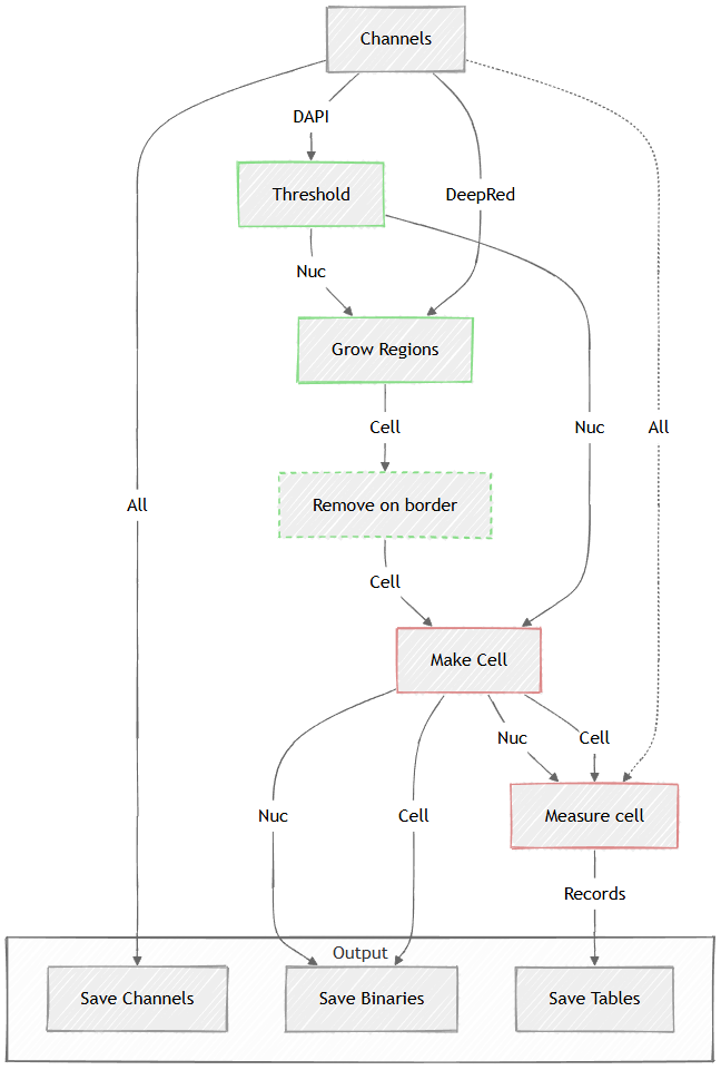
Figure 666.
Records are the products of measurements. They represent tabular data. Measurements produce records one frame at a time. In some cases the task requires bigger chunk of data at once. Hence the rows have to be accumulated over a loop or overall.
In order to display the records nicely as a table or graph chart it requires making a appropriate table or chart out of the mere records.
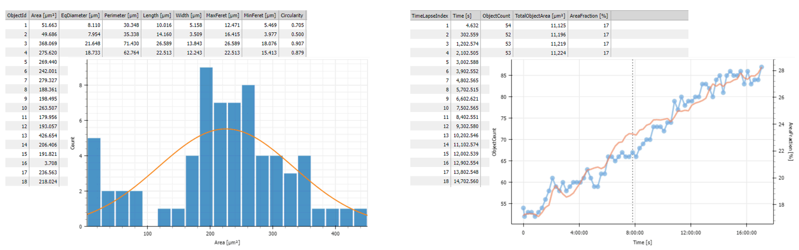
Figure 667.
It is common to show the Tables and graphs organized near the image inside panes that allow for showing and hiding the elements as needed.
In the example below the Records output of the Measurement > Basic > Object Count measurement is accumulated using Data manipulation > Basic > Accumulate Records and visualized in a Table and a Timechart showing the evolution of the number of objects over time.
The ObjTable and the Histo both contain frame data and are displayed in the left Results & Graphs > Layout > Stacked one over the other whereas the AccumTable and the Chart containing the accumulated data are displayed in the right Results & Graphs > Layout > Stacked.
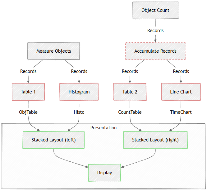
Figure 668.
Tracking objects connects the “same” objects in subsequent frames in time.
As objects appear and disappear on each frame due to nature of the sample and segmentation imperfections the “same” object typically has a different object ID on the next frame. Tracking solves this task by assigning each object a track ID which is the same for “same objects”.
The example below builds on object measurement. It combines track ID coming from the Tracking > Tracking > Track Objects with the measurement columns using Data manipulation > Basic > Append Columns (both tables have same rows – objects). The Tracking > Tracks > Accumulate Tracks puts together all the frames and organizes the Records by tracks.
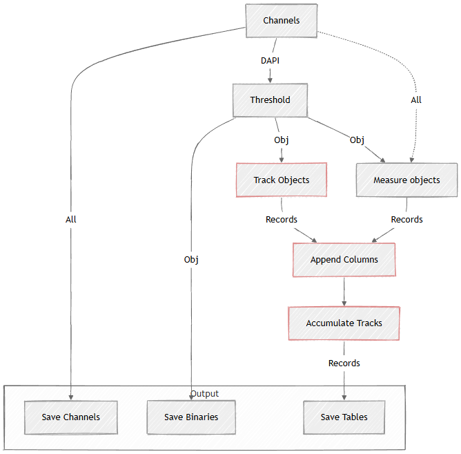
Figure 669.
Tracking particles solves the same task of assigning ID to the “same” objects. But it also measures motion features like speed.
In the example below the Tracking > Object Position > Time & Center measures time and position for every object, Tracking > Tracking > Track Particles assigns the track ID, Tracking > Tracks > Accumulate Tracks puts all particles into one record set and finally Tracking > Tracking Features > Tracking Features > Motion Features calculates the dynamics of every object.
Figure 670.