 Measurement
2D

3D
All measurements include frame metadata to be able to include time filename from the same node.
Object measurement includes all features from frame measurement, eliminating the need to add a separate field measurement node to obtain data such as the measured area.
Select the measurement feature from the Add Feature list. Click on it when you see the + symbol next to its name. It is added to the right list showing all measured features. Use the down arrow next to the feature to further specify the measurement.
If a feature displays the channels selection bar
 , first select on which channel the measurement will be done (green channel is selected in our example) and then
  add the feature. The channel can be changed later by clicking on the Change channels button next to the = icon.
Adjust the name of the feature in the Custom Name column. This name is then passed in the Analysis Results table.
Choose the Channels on which the feature is calculated.
Set the resulting Format and the number of decimal units (dec).
Child is inside the parent - all child pixels are in the parent.
Child is intersecting with the parent - they have at least one common pixel.
Child nearest parent - closest parent measured border to border.
For the count feature the presence in a compartment is defined by the position of the center pixel.
For the area and intensity features the intersection of spots and a compartment is used.
Node input/output overview for all Basic nodes.
Table 8.
| Measurement node | Input | Output |
| Field | Channel, Mast? | Row per field |
| Object | Binary, Channel* | Row per object |
| Object Count | Binary+, Channel* | Row per field |
| Parent | Parent, Child, Channel* | Row per parent object |
| Children | Parent, Child, Channel* | Row per child object |
| Cell | Cells, Nuclei, Spots?, Channel* | Row cell |
where:
? ... optional,
+ ... at least one,
* ... zero or more.
In order to reduce the number of nodes required for a recipe all nodes include features from more generic measurements. These are repeated in every row if needed. For example:
The Field node measures the intensity features in the whole image field. The output is a table where every row corresponds to one field.
Optionally, a binary input (a mask) can be connected in order to reduce the measured area. Only the pixels under the mask are measured.
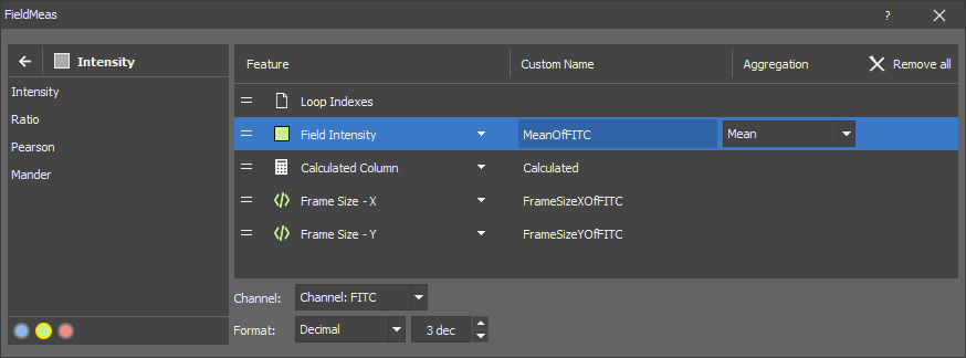
Figure 787. Field node.
All Basic measurement nodes are set in a similar way with variations in the list of measurement features depending on the node type and their dimension (2D/3D).
The  Calculator (Calculated Column) feature is different than the other features as it displays a scientific calculator at the bottom with buttons for arithmetical operations, allowing the calculation of a new column using already inserted features (click on the
  icon to insert a feature into the formula).
Measurement of some features can be further specified in their Aggregation drop-down menu. Order of a feature can be changed by clicking and dragging the feature to a different row position in the list. To hide the selected feature in the Records table, click on the  icon. To delete a feature, click on the
  icon. To remove all features in the list, click Remove all.
ObjectId and ObjectEntity are shown in the Analysis Results as {BinaryLayerName}Id and {BinaryLayerName}Entity. Naming the binary layers as Cell, Nuclei, Parent, etc., so that the columns are named CellId, CellEntity, NucleiId, etc., enhances the clarity for the user. Generally one row record is created per cell. Some nodes generate a varying number of rows compared to a classic measurement (e.g. a histogram produces one row for each pixel value or bin). Loop indexes are dependent on the input file and produce multiple columns in the analysis results table if the input file has multiple loops.
Measures all features of every object. The output is a table where every row corresponds to one object.
Optional channel inputs must be connected when intensity features are measured.
Field feature as well as field and global metadata can be measured in the same node. They are repeated for every object.
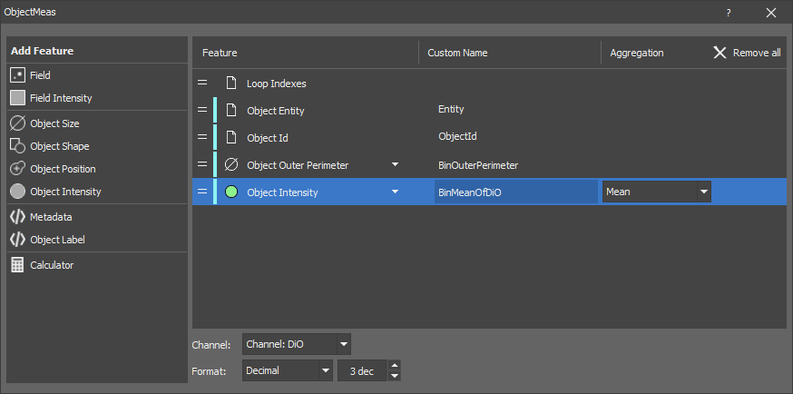
Figure 788.
The description of the dialog window behavior can be found in the Measurement > Basic > Field node.
Measures object features on the whole field. The output is a table where every row corresponds to one field.
The node measures typical binary features like Object count, Area fraction as well as all other object features as aggregates (mean, sum, max, ...).
Optionally, the node can measure more binary layers at once.
Optional channel inputs must be connected when intensity features are measured.
Figure 789.
The description of the dialog window behavior can be found in the Measurement > Basic > Field node.
Measures parent and children object features. The output is a table where every row corresponds to one parent object.
Optional channel inputs must be connected when intensity features are measured.
Parent-children relationship
Every parent may “have” zero (0) or more children. There are three methods for determining childhood:
The node measures features of the parent objects as well as aggregates (mean, sum, max, ...) of the children object features.
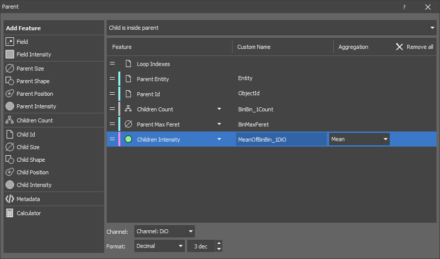
Figure 790.
Note
The Parent Id is always named ObjectId in the results. One row is created per parent. Child measurement is aggregated per parent (pick the Aggregation type for each child measurement).
The description of the dialog window behavior can be found in the Measurement > Basic > Field node.
Measures parent and children object features. The output is a table where every row corresponds to one children object.
Optional channel inputs must be connected when intensity features are measured (see Parent-children relationship in Measurement > Basic > Parent).
The node measures features of both parent and children objects. The parent features are repeated for its every child. Having all children features is useful in later downstream nodes where the parent ID can be used for grouping, reduction or sorting.
Children IDs can be “measured” and used for joining with other nested children nodes.
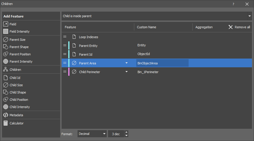
Figure 791.
Note
The Parent Id is always named ObjectId in the results. One row is created per child. Aggregation can be done using Data management > Basic > Reduce Records.
The description of the dialog window behavior can be found in the Measurement > Basic > Field node.
Measures object features of cell, nucleus and few features of the cytoplasm. The output is a table where every row corresponds to one cell and nucleus.
Optional channel inputs must be connected when intensity features are measured.
Cell must be connected to MakeCell node which ensures that every cell has exactly one. It also gives the same ID to every cell and its nucleus.
Cytoplasm is internally calculated as complement of the nucleus inside cell. Consequently it is hollow and may be split in more than one object (having same object ID though). Because of this it does not make sense to measure most of the object features.
Optionally Spots objects can be connected to count their presence in each compartment.
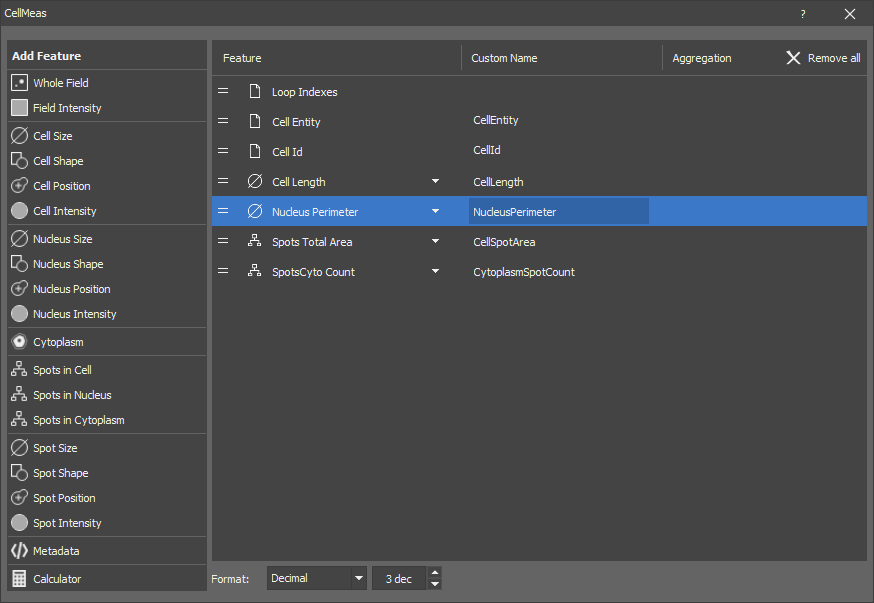
Figure 792.
Node Inputs
Layer representing cells (“Cell” output).
Layer representing nuclei (“Nucleus” output).
Layer representing “Spots” inside the nucleus or cytoplasm area.
Channel used for intensity based measured features.
The description of the dialog window behavior can be found in the Measurement > Basic > Field node.
Outputs the X and Y shift estimates (in px and µm) for the checked correction method.
Estimates the Signal to Noise Ratio (“SNR”) value present in the connected color result.
Retrieves well plate information and thumbnail using Channel A and Binaries B1, ..., Bn and stores it in the table.
Thumbnail
Defines size (in microns if calibrated) of the center portion of the frame that is cropped and rendered.
Maximum size (in pixels) is a limit to which the rendered image is stretched down if being bigger.
Labeling
List of possible labels separated by comma. Listed values are used in the “Number Of” aggregation menu (e.g. in Data management > Basic > Reduce Records node).
Calculates a histogram of all pixel values in the color image. If the connected color image has multiple channels they are averaged into a single value per pixel. If a binary is connected only pixels under it are taken.
minimum pixel value; 0 or minimum for floats by default
maximum pixel value;  or maximum for floats by default
number of histogram bins; 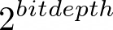 or 65536 for floats by default
Reports all pixel values of the color image. If the connected color image has multiple channels they are averaged into a single value per pixel. If a binary is connected only pixels under it are taken.
Fourier Ring Correlation (FRC) is a technique used to measure the actual resolution of two independent images of the same scene. This method produces a numerical value that represents the resolution, providing a precise and reliable measurement. However, obtaining two independent images of the identical scene can often be challenging. Despite this, FRC is versatile and applicable across various imaging modalities.
This node implements the paper Measuring image resolution in optical nanoscopy.
This node is a modification of the Measurement > Resolution > Image Pair FRC node so that it can be used for only one image and two images are not needed. This is based on the paper Fourier ring correlation simplifies image restoration in fluorescence microscopy. Accuracy and reliability is lower than on the Measurement > Resolution > Image Pair FRC node. It is calibrated for AX and NSPARC images. Trying other modalities is not recommended.
Calculates histogram of all pixel values for every binary object.
Please see Measurement > Field pixel values > Histogram.
Calculates histogram of all voxel values for every binary object.
Please see Measurement > Field pixel values > Histogram.
Reports all pixel values along every line. If the object is not a line the order of pixel is undefined.
Calculates entropy of voxel values for every binary object.
Calculates sample kurtosis of voxel values for every binary object.
Calculates the maximum intensity for each object in the connected color result under the connected 3D binary result. Please see MaxIntensity .
Calculates the mean intensity for each object in the connected color result under the connected 3D binary result. Please see MeanIntensity .
Calculates the minimum intensity for each object in the connected color result under the connected 3D binary result. Please see MinIntensity .
Calculates quantile in the connected color result for each 3D object present in the connected 3D binary result. Please see Measurement > Field intensity > Quantile.
Calculates sample skewness of voxel values for every binary object.
Calculates the standard deviation of intensity for each 3D object (“StDevIntensity”) in the connected color result under the connected 3D binary result.
Calculates the sum of intensity in every voxel of the connected color result (“SumIntensity”) under the connected binary result for each object separately. Please see SumIntensity .
Shows the intensity variance for each 3D object in the connected color result under the connected 3D binary result.
Calculates uniformity of color voxel values for every binary object.
Measures the smallest distance to another 2D/3D object. Please see NearestObjDist .
Calculates the distance between objects in two binary layers.
calculates distance between the centers of two objects.
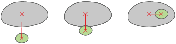
Figure 793.
calculates distance between the center of one object and the closest point on the border of the other object.
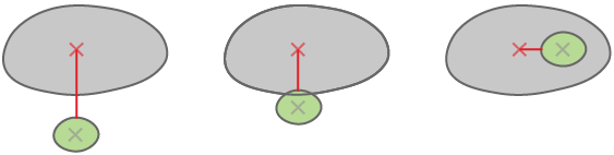
Figure 794.
calculates distance between the borders of objects (minimal distance between borders). When the objects are touching, the distance is 0.
Figure 795.
Measures one or more field features.
See the dedicated documentation: Extending GA3.
Measures one or more object features.
See the dedicated documentation: Extending GA3.
Calculates the focus criteria (values which estimate the image sharpness) for each slice in a Z-stack and estimates the focus position. For the bright field and fluorescence criteria, the x-y region of the image is divided into 3x3 crops. The focus criterion is calculated for each crop and Z-position, and the overall results are used to estimate the focus position. The calculated focus position corresponds to the value that would be obtained during (non-AI) live auto-focusing if the camera captured the same Z-stack.
Choose the type of the focus criterion.
Choose how the focus should be evaluated as if the Z-stack was obtained in one of the following modes: Single pass autofocus (Single pass), first pass of two-pass (2 passes: pass #1) autofocus, or second pass of two-pass autofocus (2 passes: pass #2).
Output columns
Z-position of each slice.
Validity of the focus estimation. Can be either OK (the focus position was found), Small range (the focus position is out of range) or Fail (focus position couldn't be estimated).
If the result of the validity check was OK, this column contains the found focus position. If the focus was found to be out of the Z-range, it contains the Z-value at the corresponding border of the range. If the focusing failed, it contains nothing.
Focus criteria calculated across Z for the whole image.
Focus criteria calculated across Z for each crop. Crops #1 - #3, #4 - #6 and #7 - #9 correspond, respectively, to the top, middle and bottom of the image.
If the result is OK, this column contains the focus criteria calculated across Z for the crop which had the most impact on the Z-position. Otherwise, this column is empty.
Shows the total volume of all objects present in the connected binary result.
Volume of the objects in the connected binary result is divided by the total volume of the analysed image.
Calculates Costes Background of all voxel values. If the connected color volume has multiple channels they are averaged into a single value per volume. If a binary is connected only voxels under it are taken into account.
It is a background estimation of two channels based on the Costes method. This method assumes that the correlation of values in both channels should be zero for background pixels. It is used mainly in colocalization analyses.
Calculates entropy of all voxel values. If the connected color volume has multiple channels they are averaged into a single value per voxel. If a binary is connected only voxels under it are taken.
Please see Measurement > Field intensity > Entropy.
Calculates sample kurtosis of all voxel values. If the connected color volume has multiple channels they are averaged into a single value per voxel. If a binary is connected only voxels under it are taken.
Please see Measurement > Field intensity > Kurtosis.
Calculates histogram of all voxel values. If the connected color volume has multiple channels they are averaged into a single value per voxel. If a binary is connected only pixels under it are taken.
Please see Measurement > Field pixel values > Histogram.
Finds maximum voxel value in every object. If the connected color volume has multiple channels they are averaged into a single value per voxel. If a binary is connected only voxels under it are taken.
Calculates arithmetic mean of all voxel values. If the connected color volume has multiple channels they are averaged into a single value per voxel. If a binary is connected only voxels under it are taken.
Please see Measurement > Field intensity > Mean.
Finds minimum voxel value. If the connected color volume has multiple channels they are averaged into a single value per voxel. If a binary is connected only voxels under it are taken.
Finds voxel value that appears most often. If the connected color volume has multiple channels they are averaged into a single value per voxel. If a binary is connected only voxels under it are taken.
Please see Measurement > Field intensity > Mode.
Calculates n-th quantile of all voxel values. If the connected color volume has multiple channels they are averaged into a single value per voxel. If a binary is connected only voxels under it are taken.
Please see Measurement > Field intensity > Quantile.
Calculates sample skewness of all voxel values. If the connected color volume has multiple channels they are averaged into a single value per voxel. If a binary is connected only voxels under it are taken.
Please see Measurement > Field intensity > Skewness.
Calculates sample standard deviation of all voxel values. If the connected color volume has multiple channels they are averaged into a single value per voxel. If a binary is connected only voxels under it are taken.
Please see Measurement > Field intensity > Standard Deviation.
Calculates sum of all voxel values. If the connected color volume has multiple channels they are averaged into a single value per voxel. If a binary is connected only voxels under it are taken.
Please see Measurement > Field intensity > Sum.
Calculates uniformity of all voxel values. If the connected color volume has multiple channels they are averaged into a single value per voxel. If a binary is connected only voxels under it are taken.
Please see Measurement > Field intensity > Uniformity.
Calculates sample variance of all voxel values. If the connected color volume has multiple channels they are averaged into a single value per voxel. If a binary is connected only voxels under it are taken.
Please see Measurement > Field intensity > Variance.
Calculates the volume center (X, Y, Z in µm) of the connected color image.
Calculates the volume center (X, Y, Z in px) of the connected color image.
Gives access to the metadata such as Exposure Time, Plate Name, Well Row, Slide Barcode, etc.
Calculates the mean of ratios between corresponding pixels of the two input channels (nominator, denominator) under the input binary mask in 3D.
Calculates Pearson correlation coefficient for a volume image. For more information please see Measurement > Object ratiometry > Pearson Coeff.
Calculates Manders overlap for a volume image. For more information please see Measurement > Object ratiometry > Manders Coeff.
Calculates the Equivalent Diameter (“EqDiameter”) for each 3D object in the connected binary result. It represents a sphere with the same volume as the measured object. For more information please see EqDiameter .
Calculates the volume of each object in the connected 3D binary result.
Calculates the surface of each 3D object in the connected binary result.
Note
Computation method of this node is based on David Legland: Computation of Minkowski Measures on 2D and 3D binary images. DOI: 10.5566/ias.v26.p83-92.
Calculates the Major Axis Length for each object in the connected 3D binary result. Please see Major Axis Length.
Calculates the Minor Axis Length for each object in the connected 3D binary result. Please see Minor Axis Length .
Calculates the Minor 2 Axis Length for each object in the connected 3D binary result. Please see Minor2 Axis Length .
Calculates the elongation of each object in the connected 3D binary result. Please see Elongation .
Please see Measurement > Object ratiometry > Pearson Coeff.
Please see Measurement > Object ratiometry > Manders Coeff.
Defines the child/parent emplacement and specifies which records from the connected nodes are shown. Order of the records can be changed by the arrow buttons.
This node uses aggregation statistics. Please see Data management > Grouping > Aggregate Rows and Measurement > Object parenting > Aggregate Children.
Please see Measurement > Object parenting > Child Distance.
Please see Measurement > Object parenting > Nearest Child.
Measures the inserted 3D features using the parent-child hierarchy. Use the first drop-down menu to select the hierarchy corresponding to your sample (Child is inside parent, Child is intersecting parent or Child's nearest parent). Then add feature(s) to be measured.
Please see Measurement > Object parenting > Parent Distance.
Shows the X, Y and Z distance from the top left corner to the center of gravity of each object.
Shows the X, Y and Z distance in pixels from the top left corner to the center of gravity of each object.
Shows absolute coordinates of the center of gravity of each object in the scope of the stage XYZ range.
Shows the X, Y and Z coordinate of the object's centroid in pixels.
Shows absolute coordinates of the centoid of each object in the scope of the stage XYZ range.
Shows the bounds of each 3D object in pixels. Please see BoundsPxLeft .
Shows the absolute bounds of each 3D object. Please see BoundsAbsLeft .