 Image Processing
Deconvolution

Background
Contrast
Convolution
Denoising
Detection
Insert
Morphology
Linear Morphology
Linear Morphology 3D
Labels & Classes
Transformations
JavaScript
Image intensity (signal is Bright)
Ball of the defined radius
Estimated background
Light Background (Brightfield)
Black Background (Fluorescence)
Average Background (DIC, PhC)
Light Background (Brightfield) - for Brightfield
Black Background (Fluorescence) - for Fluorescence
Average Background (DIC, PhC) - for Differential Interference Contrast or Phase Contrast
Smooth
Vertical Edges
Horizontal Edges
Edges
![]()
Please see 2D Deconvolution for more information about deconvolution.
Performs the automatic shading correction. Choose the type of correction which best represents your image background.
This function estimates the background intensity by rolling a ball of the defined radius over/under the image intensities.
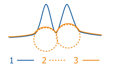
Figure 900. Rolling Ball Background Correction Scheme
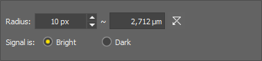
Figure 901.
Set radius in pixels. The value should be bigger than size of the biggest object in the image.
Choose signal intensity - Bright for fluorescence images, Dark for bright-field images.
This command defines parameters of the background shading correction.
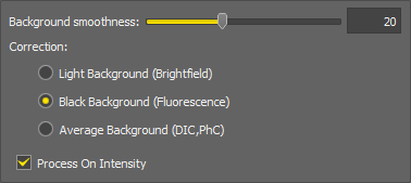
Figure 902.
Defines the smoothness of the curve estimating the background. The lower the number the more smooth the curve is. With higher numbers the local changes become more accented.
Select on which background the correction is performed:
See also Acquire > Shading Correction Panel.
Performs the background shading correction only inside the ROI (Region Of Interest) area.
Select on which background the correction is performed:
See also Acquire > Shading Correction Panel.
Subtracts the background of the connected image using the connected binary mask. Select the category of information that the mask contains (Background or Objects).
Subtracts a value from the connected result. Fill the value to be subtracted in the edit box.
Compensates image shading of the current image using a correction image specific for Confocal Microscope AX. Adjust the Strength using the slider.
Enhances contrast of the connected result automatically based on the Low/High values.
Pixels with an intensity less than Low are set to zero.
Pixels with an intensity greater than High are set to 255.
Increases contrast of the image. It changes intensities of the current image. Hue and saturation are not affected. Intensities are rescaled according to the selected method.
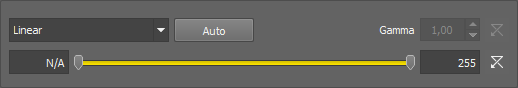
Figure 903.
Options
Sets the Range so that the limits correspond to the minimum and maximum intensities found in the image.
The parameter for the Gamma Correction method. It ranges from 0.05 to 5.00. Set Gamma < 1 to get more information in dark areas or set Gamma > 1 to enhance bright parts of the image.
Set the low/high contrast intensities. Pixels with intensity greater than the high value set will be changed to a pure white, whereas pixels with intensity smaller than the low value set will be changed to pure black (zero). The range itself will be stretched to fit the available intensity range.
Closes the dialog window and applies the contrast settings.
Closes the dialog window without applying the contrast settings.
Opens this help page.
Turns the preview on/off.
Methods
These transformations stretch the intensity interval defined by the range to the full intensity range using the selected curve. All values outside the range are set to pure black and pure white.
Equalization transformation leads to uniform intensity distribution in the specified interval <Low, High>.
Gamma correction maps the intensity interval <Low, High> according to exponential equation with the gamma parameter.
This command increases sharpness of the image. However, the scale in which the sharpening is performed is bigger than standard - i.e. large objects are affected, not tiny details.
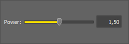
Figure 904.
Set the power value. The possible range of values is from 1.01 to 2.
Sets the default value to the power text box. The default value is 1.25.
Enhances contrast of the current image while accentuating its details. The contrast is enhanced within both bright and dark areas of the image.
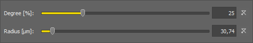
Figure 905.
Contrast multiplicator which is locally proportional to contrast amplification.
Size of the neighborhood to be processed.
This function sharpens the image.
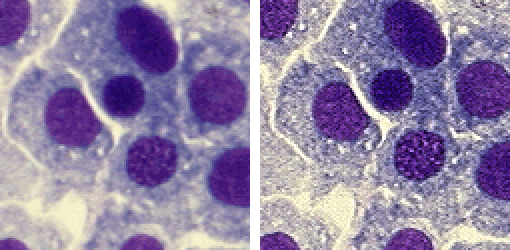
Figure 906. Before - after applying the Sharpen function
This function slightly sharpens the image.
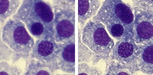
Figure 907. Before - after applying the Sharpen Slightly function
Enhances details on the alpha channel (Alpha) and the standard channel (Details) and removes the noise which originates in the detail enhancement (Noise).
Sharpens the image using the unsharp masking technique.
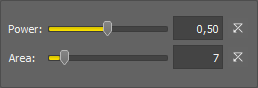
Figure 908.
Set the strength of the sharpening effect. The possible range of values is from 0.01 to 1.
Define the area size which is used during calculating the result. The larger the area is, the smoother the result will be.
Convolves the image with the selected common filter.
Edge detection (en.wikipedia.org/wiki/Sobel_operator)
Edge detection (en.wikipedia.org/wiki/Prewitt_operator)
Applies standard Gaussian filters to the color image. The result is a floating point image.
Blurs the image.
First derivative. Detects (emphasizes) edges in the specified axis direction.
Second derivative. Detects (emphasizes) edges in the specified axis direction.
Parameter σ (dispersion) for the Gaussian filter. For the basic Gaussian filter, it determines extent of the blur. For the other filters, it determines the size of edges that are going to be detected.
Smooths and detects edges of color image.
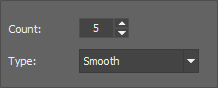
Figure 909.
Number of steps used in the algorithm.
Type of filter.
Note
Golay filter function uses polynomial (second order) fitting of the image data for smoothing image. Fitting is performed in the neighborhood defined by Kernel parameter. The Vertical Edges detection is derived from the 1st derivation of image data in the X direction. The same is true for Horizontal Edges detection (Y direction). General edge detection is calculated as the sum of the absolute values of the 1st derivations in X and Y directions. Edge detection includes dynamics corrections. Algorithm exactly calculates edge values.
This function performs filtration on intensity component (or on every selected component - when working with multichannel images) of an image using convolution with 5x5 kernel. Mexican Hat kernel is defined as a combination of Laplacian kernel and Gaussian kernel, it marks edges and also reduce some noise.
Denoising action can be used to reduce any kind of noise in the image (Gaussian, Poisson noise). The described neighborhood is 3 dimensional - i.e. information is taken from the neighboring frames.
Original method is based on denoising via pixel large neighborhoods in a spatial and frequency (incl. wavelets coefficients) meaning. It is a one-pass algorithm.
Regression algorithm iteratively denoises every pixel according to its local neigborhood. In every iteration, local linear regression is computed for every pixel and the value is replaced by the regressed value. This method belongs to the same family as the Original method.
Fusion method is a fusion between Original and Regression. It takes the better parts of both algorithms.
Bayes method is slow, but it uses a high-quality algorithm. A probabilistic approach is used to compute the most likely estimate from the neighboring pixels.
Iterative prediction is very similar to the Regression method but in the new iteration, we find a new value by voting from extrapolation of neighboring pixels.
Define the strength of the denoising algorithm for each channel separately using the slider or the edit box. If the slider is set to zero, denoising is done with an estimated noise variance. Move the slider to the right and denoising calculates with higher noise variance (more noise is present in the image) and vice versa.
Fast denoising works the same as Image Processing > Denoising > Denoising with the exception that described the neighborhood is 2 dimensional - i.e. information is taken only from the current frame.
Removes stripes created by the VisiTech iSIM device.
Defines the strength of the stripe removing.
This command defines a filter, which passes only details larger than the set pixel value.

Figure 910.
Set the size of details which will be kept. Smaller details will be suppressed.
This function filters small irregularities in images.
Select the size of neighborhood used for Median filtering.
 Reset
Reset Sets the dialog default values.
This command performs smoothing on the color image.
Click the button to change the structuring element used for this operation. See Matrix.
Number of iterations.
Reset Sets the dialog default values.
Approximation of the standard Gaussian filter. Results should be similar to Image Processing > Convolution > Gaussian Filters, but faster.
Parameter σ (dispersion) for the Gaussian filter. For the basic Gaussian filter, it determines extent of the blur.
This command can enhance objects in a DIC image so that the objects can be thresholded reasonably.
The Differential interference contrast capturing method produces special kind of images, where objects look three-dimensionally having glow on one side and shadow on the other side. Such objects can not be thresholded and further analysed. The Detect DIC Objects command performs recognition of the objects and makes them bright in order to be easily thresholded.
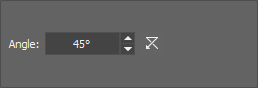
Figure 911. Detect DIC Objects dialog for Multichannel images
Specify the angle of illumination in the edit box.
Detects and highlights filament structures present in the connected color image (e.g. neurons, blood vessels, ...). Set the diameter range of the filaments in your sample, set how many times this range is evaluated (Steps) and enhance the result using Contrast.
Detects and highlights 3D filament structures present in the connected color image with a Z dimension (e.g. neurons, blood vessels, ...). Set the diameter range of the filaments in your sample, set how many times this range is evaluated (Steps) and enhance the result using Contrast.
Gabor Edge Detection method represents a linear filter useful for visualizing specific features of an image. Use the Orientation combo box to select a direction [°] in which the features are visualized. Select a proper direction and adjust the Amplitude of the wavelet to find the sharpest result. Real, Imaginary or Both filters can be applied. Switching from Positive to Negative Value highlights the surroundings of the object.
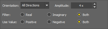
Figure 912.
Select a direction in degrees in which the features are visualized.
Adjust the amplitude of the wavelet to find the sharpest result.
Apply one of the filters or both.
Switching from Positive to Negative highlights the surroundings of the object.
Detects edges by morphological transformations of color images.
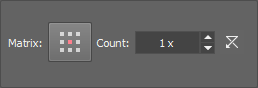
Figure 913.
Click the button to change the structuring element used for this operation. See Matrix.
Number of iterations.
Reset Sets the dialog default values.
Note
Morphologic gradient is the difference between dilated and eroded images. It enhances edges.
Click the button to change the structuring element used for this operation. See Matrix.
Number of iterations.
Reset Sets the dialog default values.
Note
Detect Peaks command enhances small light objects by “Top Hat” morphologic transformation. The size of objects selected is determined by the size of the used structuring element, which depends both on Matrix and Number parameters. This command enables the specific segmentation of small objects to the exclusion of larger objects and also can help you in the case of non-homogeneous background.
Detects regional maxima. It is a subset of top hat transformations.
Click the button to change the structuring element used for this operation. See Matrix.
Number of iterations.
Reset Sets the dialog default values.
The Regional Minima function detects regional minima. It is a subset of top hat transformations.
Click the button to change the structuring element used for this operation. See Matrix.
Number of iterations.
Reset Sets the dialog default values.
Detects edges by morphological transformations on color images.
Click the button to change the structuring element used for this operation. See Matrix.
Number of iterations.
Reset Sets the dialog default values.
Note
The Detect Valleys command enhances small dark objects by “Top Hat” morphologic transformation. The size of the selected objects is determined by level of the transformation, which depends on Matrix type and on Number of steps. This command enables the specific segmentation of small objects to the exclusion of larger objects and also can help you in the case of non-homogeneous background.
Inserts a grayscale color gradient over the connected image. The gradient is defined by a gradient table where the first column sets the color change points and the second column defines the color of the segment (0 = black, 1 = white). Use decimals to set a specific change position or shade of gray. Angle of the gradient can be adjusted optionally.
Performs morphological opening on current color image. Morphological opening is erosion followed by the same number of dilations. The transformation removes small light objects. If the structuring element dimension has an odd value, there are two enhanced pixels in structuring element depicting centers: one for erosion and the other for dilation.
Figure 914.
Click the button to change the structuring element used for this operation. See Matrix.
Number of iterations.
Reset Sets the dialog default values.
Performs morphological closing on the current color image.
Figure 915.
Click the button to change the structuring element used for this operation. See Matrix.
Number of iterations.
Reset Sets the dialog default values.
Morphological closing is a dilation followed by the same number of erosions. Small dark areas are removed by this transformation. If the structuring element dimension has an odd value, there are two enhanced pixels in structuring element depicting centers: one for erosion and the other for dilation.
Performs morphologic erosion on color image. Erosion affects the intensity of color image. Hue and saturation are not affected. Dark areas grow whereas light areas shrink.
Figure 916.
Click the button to change the structuring element used for this operation. See Matrix.
Number of iterations.
Reset Sets the dialog default values.
See Also
Image > Morphology > Open Image > Morphology > Open, Image > Morphology > Close Image > Morphology > Close, Image > Morphology > Dilate, Image > Morphology > Linear Erode
Performs morphological dilation on color image. Dilation of color images changes their intensity. Light areas grow and small dark objects and structures disappear. Hue and saturation are not affected.
Figure 917.
Click the button to change the structuring element used for this operation. See Matrix.
Number of iterations.
Reset Sets the dialog default values.
Fills holes in the connected color image. Holes which are connected to image borders remain intact.
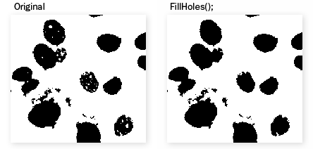
Figure 918. Example
Removes small light areas in the direction specified by Matrix.
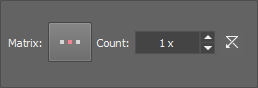
Figure 919.
Click the button to change the structuring element used for this operation. See Matrix.
Number of iterations.
Reset Sets the dialog default values.
Closes color image using a linear structuring element.
Figure 920.
Click the button to change the structuring element used for this operation. See Matrix.
Number of iterations.
Reset Sets the dialog default values.
Note
Linear morphological closing is a dilation followed by erosion using the same linear structural element. The transformation is performed on the intensity component and removes small dark areas in the direction specified by Matrix orientation. Number specifies level of closing.
Erodes color image using a linear structuring element.
Figure 921.
Click the button to change the structuring element used for this operation. See Matrix.
Number of iterations.
Reset Sets the dialog default values.
Note
Linear erosion affects the intensity of color image in one direction. Hue and saturation are not affected. Dark areas linearly grow whereas light areas linearly shrink in the direction defined by Matrix orientation. It is an anisotropic transformation.
Erodes color image using a linear structuring element.
Figure 922.
Click the button to change the structuring element used for this operation. See Matrix.
Number of iterations.
Reset Sets the dialog default values.
Note
Linear dilation of color images changes their intensity in one direction, specified by Matrix orientation. Light areas linearly grow and small linear dark objects and structures disappear. Hue and saturation are not affected. It is an anisotropic operation.
Highlights structures with a linear pattern using the Linear Open function in the Z direction. Please see Image Processing > Linear Morphology > Linear Open.
Highlights structures with a linear pattern using the Linear Close function in the Z direction. Please see Image Processing > Linear Morphology > Linear Close.
Highlights structures with a linear pattern using the Linear Erode function in the Z direction. Please see Image Processing > Linear Morphology > Linear Erode.
Highlights structures with a linear pattern using the Linear Dilate function in the Z direction. Please see Image Processing > Linear Morphology > Linear Dilate.
This node is used to smooth out rough patches of classes. For every pixel it evaluates the surrounding area and takes the most frequent pixel.
Size of the computation element.
Adds grayscale color borders to the connected image. Enter the border size [px] for each side (Top, Left, Right, Bottom) and enter the color value (0=black, 255=white).
Reduces size of the input image based on the binning factor and binning method.
Binning factor of 3x3 will reduce the area of 9 pixels into a single pixel in the resulting image based on the selected method.
The resulting pixel value will be calculated as maximum, minimum, mean or sum. Sum No Noise method brightens the image but does not amplify noise like the sum method does.
Crops the connected image to the specified width and height [px]. Shift the cropping rectangle by filling the Start x and Start y position.
Crops to the center of the connected image by the specified width and height [px].
Shrinks the source image so that it fits into a square with a given size. Aspect ratio of the image is maintained as well as all other properties.
Number of pixels of the longer side of the image.
Interpolation method used for rescaling.
Flips the source image horizontal and/or vertical. Simply check Horizontal flip or Vertical flip to flip the image in the particular direction.
Shifts the connected color image horizontally (X Offset) or vertically (Y Offset). Area shifted outside the image borders can be placed to the opposite side if Rotate values around image borders is checked.
Resizes the image by a given ratio.
Ratio in X axis.
Ratio in Y axis.
Interpolation method used for rescaling.
Resizes the source image (A) so that it has the same size as the reference image (B).
Interpolation method used for rescaling.
Transforms source color image into the resulting color image. The transformation is to be programmed in JavaScript.
See the dedicated documentation: Extending GA3.
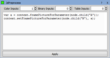
Figure 923.
See the dedicated documentation: Extending GA3.
Transforms source color image into the resulting float image. The transformation is to be programmed in JavaScript.
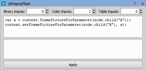
Figure 924.
See the dedicated documentation: Extending GA3.