Run the  Deconvolution > 2D Deconvolution command to display the following window.
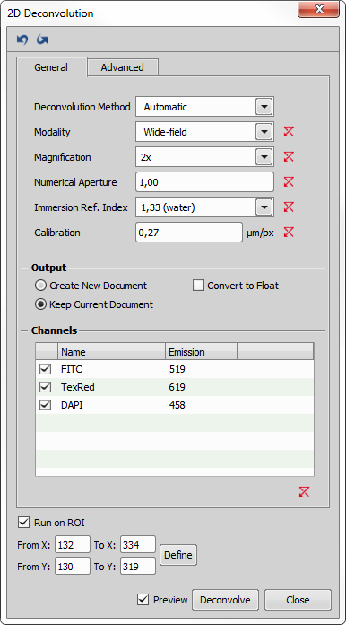
Figure 612.
Dialog window settings

 Undo/Redo
 These buttons implement a standard undo/redo functionality.
Select which deconvolution method is applied. See Deconvolution methods for further details.
To handle the out-of-focus planes correctly, it is important to know how exactly the image sequence has been acquired. Select the proper microscopic modality from the combo box.
Depending on the Modality setting, set the pinhole/slit size value and choose the proper units.
If SFC/Slit mode is selected in the Modality field, define the slit orientation (horizontal, vertical).
Enter refraction index of the immersion medium used. There are some predefined refraction indexes of different media in the nearby pull down menu.
Specifies whether a new document showing the deconvolved image is created (Create New Document) or the current image is overwritten with the result of the deconvolution process (Keep Current Document). Convert to Float option enables the user to convert 3D deconvolved images into floating point image. When Create New Document is checked, this conversion is done automatically.
Specify an estimation of the amount of noise present in the image.
Note
For the Richardson-Lucy deconvolution method a precise SNR (signal to noise ratio) value can be entered into the edit box when Custom noise level is selected. This value ranges from 1 (noisy image) to 50 (image almost without noise).
For the Richardson-Lucy, Landweber and Blind deconvolution methods an Automatic noise level recognition can be set.
Blind, Landweber and Richardson-Lucy deconvolution are iterative methods. More iterations (repetitions) take more computation time but usually improve quality of the result. Specify the number of iterations.
Note
For the Richardson-Lucy and Landweber deconvolution methods an automatic recognition of number of iterations can be turned on (Auto Stopping).
Estimate thickness of the specimen: Flat, Thin, Normal, or Thick. This parameter influences the PSF shape.
Enables the user to import the Point Spread Function image. If this is done, the deconvolution parameters will be disabled.
Importing PSF can be of great help especially if you have determined the PSF image by capturing a nano-bead. It is reasonable to import the PSF for fast, blind and Richardson-Lucy deconvolution either. See Determining the Point Spread Function (PSF).
Multiple point spread functions can be imported at once if previously extracted from different layers by the Deconvolution > Extract PSF command. The deconvolved Z dimension is then divided into the appropriate number of segments. Each PSF is applied to the corresponding segment (e.g. 3 layers = 3 unique PSF – for the top, middle and bottom part of the deconvolved Z-stack).
Image channels produced by your camera are listed within this table. You can decide which channel(s) shall be processed by checking the check boxes next to the channel names. The emission wavelength value may be edited (except the Live De-Blur method).
Note
Brightfield channels are omitted automatically.
This function can be used to subtract the background value from the image, deconvolution process is performed on the image without the background and once the process is finished, the background is placed back into the deconvolved image to its original place. By default the function is turned off (Do not subtract). Average background value can be estimated automatically (Subtract automatically) or defined manually (Subtract manually). When defining background manually, the Background Picker dialog window appears after clicking (see: Define Background).
Note
This option works on the sample, not on the PSF.
If turned on, spherical aberration of the PSF is calculated and used. Enter the Acquisition Depth (depth defining the center of the sample where the PSF is generated). Default value of the Acquisition Depth is taken from image metadata as a distance from the Z-Stack edge to the Z-Stack Home position. This distance is in most cases 1/2 of the Z-Stack depth. The only exception is the Asymmetric Z-Stack mode where the home position is explicitly defined by the experiment setting.
Adjust the number of Layers if you want to use the depth variant deconvolution. If you set Layers to a number bigger than one, the stack is internally split in the Z dimension into several sub-stacks (layers) and an aberrated PSF is computed separately for each one. For example a Z stack having a total range of 10 µm, 5 layers, and acquisition depth (set in the deconvolution dialog) of 10 µm will generate PSFs for the sub-volumes at 6 µm, 8 µm, 10 µm, 12 µm, and 14 µm.
Finally set the Sample Refractive Index value (refractive index of the medium used for sample acquisition). Default Sample Refractive Index is 1.35 (for water).
If Use Spherical Aberration Correction is turned off, PSF without any aberration is used.
Automatically computes the PSF.
Enables the user to import the Point Spread Function image. If this is done, the deconvolution parameters will be disabled.
Importing PSF can be of great help especially if you have determined the PSF image by capturing a nano-bead. It is reasonable to import the PSF for fast, blind and Richardson-Lucy deconvolution either. See Determining the Point Spread Function (PSF).
Multiple point spread functions can be imported at once if previously extracted from different layers by the Deconvolution > Extract PSF command. The deconvolved Z dimension is then divided into the appropriate number of segments. Each PSF is applied to the corresponding segment (e.g. 3 layers = 3 unique PSF – for the top, middle and bottom part of the deconvolved Z-stack).
Deconvolution can be performed just on a portion of the image - region of interest. Check Run on ROI and define the ROI parameters. Click to draw the ROI directly into your image and confirm it by clicking the secondary mouse click. Or fill in the rectangle values manually into the edit boxes. enters the maximal Z stack range.
Displays a preview image of the current settings.
Note
When computing the preview image, deconvolution is applied to the current view. For example, having a mono timelapse ND file, the deconvolution is applied to the currently displayed frame. Total time needed for deconvolution of the whole file can be then estimated as Preview Time x Number of Time Frames. If you process a single-frame image, the preview time equals the deconvolution time.