
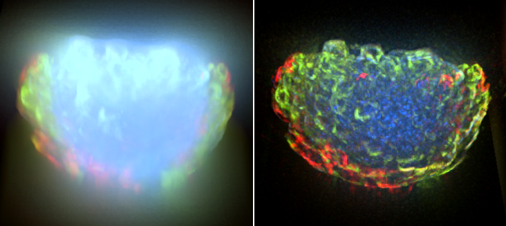
Figure 572. 3D volume data before and after deconvolution
There are different ways to sort deconvolution methods, either by the image data to be processed (2D/3D) or by the method of PSF determination (blind, Richardson-Lucy), or by expected quality of the result (fast). There are several commands available within the Deconvolution pull-down menu. Read the following overview and decide which command best suits your requirements:
Deconvolution Commands
 Deconvolution > 3D Deconvolution
 (requires: 3D Deconvolution) This command is designed to work strictly with volume data-sets i.e. ND2 files containing Z-stack.
Deconvolution > 2D Deconvolution (requires: 2D Deconvolution) Standard 2D single-frame images or ND2-files (Timelapse, multipoint, Z-stack...) can be processed by this command.
Note
Frame-by-frame deconvolution is performed in this case. Z-stack ND2 file can be processed by this deconvolution method as well, but the result will not be as good as you get from the 3D method.
Deconvolution > Show Live De-Blur Setup Deconvolution of the live image may be performed by this command. A control panel appears where its parameters can be set and the processing on live image can be turned on/off.
Deconvolution methods
It is possible to decide between the following deconvolution methods. Each method uses a different algorithm to achieve the same goal (see Algorithms).
It is stable method which produces good results.
It is faster than blind deconvolution.
It reduces image noise efficiently.
It produces decent results even if you do not import PSF.
The results may have lower contrast compared to the Blind deconvolution.
Some image details may remain blurry.
It is the fastest method (compared with Blind and Richardson-Lucy methods).
It is stable (little less than the Richardson-Lucy method).
It produces excellent results (not as bright as Blind in most cases, but with significantly less noise, which makes sample structures more clear).
Needs approximately the same memory as Richardson-Lucy method.
Rarely diverges.
It produces top quality results.
It makes very precise estimation of the PSF shape.
It enhances even the smallest image details.
The strength of this method may amplify image noise.
In some cases, the method might diverge and give unsatisfactory results.
It is super fast
Despite its swiftness, it can produce good results.
The results are not as good as from the other methods.
It can add artifacts to the image.
Stable on big images which need to be split for computing on GPU.
Robust in the presence of noise.
Good modeling of background in images.
Improved handling of image boundaries.
Slower processing speed.
Sensitive to noise level and background level settings.
This method automatically deconvolves the opened image based on an analysis of its noise characteristics, background presence and metadata. It is equivalent to running the Richardson-Lucy method with automatic noise level, auto stopping and a maximum number of iterations according to the following table:
Table 12.
| 3D widefield | iterations = 90 |
| 3D other than widefield | iterations = 60 |
| 2D widefield | iterations = 120 |
| 2D other than widefield | iterations = 60 |
Using Richardson-Lucy deconvolution assumes we know the PSF exactly, so the system does not have to estimate it (see Determining the Point Spread Function (PSF)). This type of deconvolution usually leads to reliable results.
Landweber deconvolution is a current state-of-the-art method based on wavelet deconvolution. It can deal with noise and deliver crystal clear results.
This deconvolution method estimates the shape of the PSF from the parameters specified within the deconvolution dialog window. However, if the known PSF is used, it further improves the final result. Concerning RAM usage, it is the most demanding of all the methods.
This method is optimized for speed.
Robust and versatile method where the deconvolution problem is formulated as an energy functional problem and numerically solved by a regularized minimization of it.
Note
This method is more sensitive to the background subtraction settings. We do not recommend choosing the Do not subtract option in the Preprocessing section of the Advanced tab.
Advantages
Disadvantages
A more complex algorithm based on MAP. It analyzes the image and automatically determines the optimal noise level as well as the number of iterations. For suitable widefield images (typically 3D data with a low level of noise), it also uses a faster MAP variant, which is roughly 4x faster than the standard MAP method.
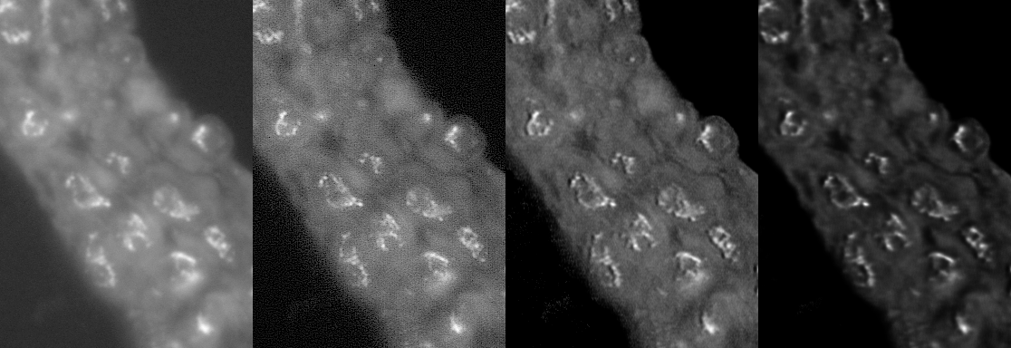
Figure 573. Comparison of deconvolution methods, from left: original image, fast, Richardson-Lucy, blind
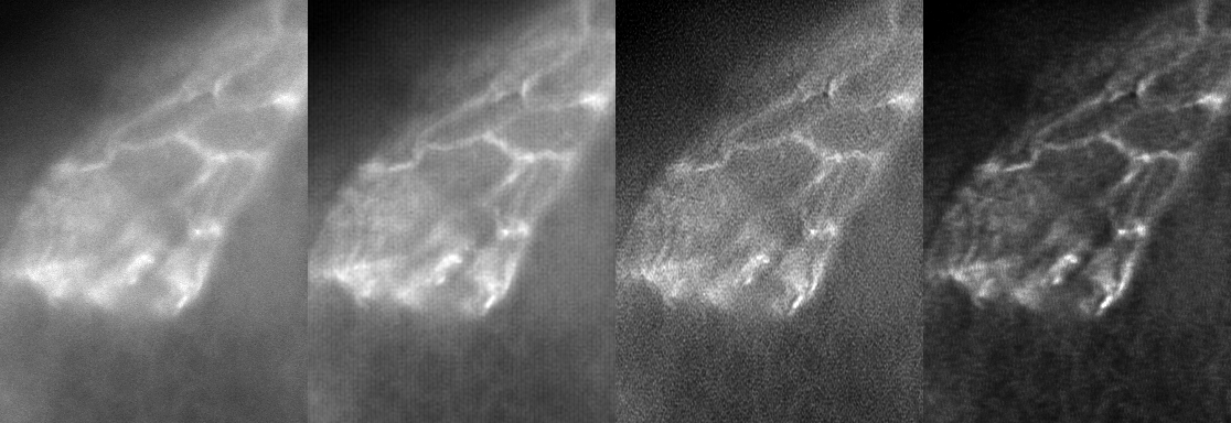
Figure 574. Comparison of deconvolution methods, from left: original image, fast, Richardson-Lucy, blind
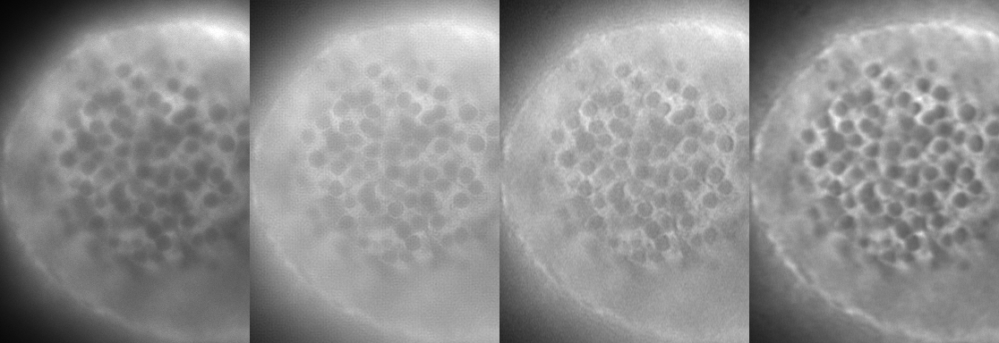
Figure 575. Comparison of deconvolution methods, from left: original image, fast, Richardson-Lucy, blind