Our model representing observed image is:

In this equation, (b) is the observed image, (A) is a general transformation matrix and (w) is additional noise. We define the following problem to solve

where (λ) is parameter of the regularization term – L1 norm of x. We can restrict matrix (A) from its generality to represent only the space invariant convolution to solve the problem efficiently. The minimization leads us to a two step algorithm.

Repeat until the convergence is reached:

This algorithm is called ISTA and converges quite slowly. There exist many improvements of the algorithm with faster convergency. Here are some of them: TwISTA, SISTA, FISTA, FWISTA. Our Landweber method uses FWISTA.

This method is an implementation of the Accelerated Lucy-Richardson algorithm with noise regularization. It is assumes that the input PSF parameters are known accurately. The problem which we try to solve can be described by the following equation:

We know the captured image (C) and the PSF (B). We look for the true image (A) and we know there it is some additional noise (N) present. The * operator stands for convolution. So the equation can be rewritten as:

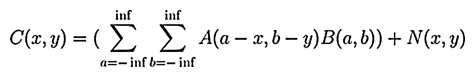
The Lucy-Richardson (LR) algorithm belongs to the class of so-called Expectation Maximization(EM) algorithms where we assume the noise(N) has a Poisson distribution. We don't need any other characteristics of N. This algorithm estimates A from given B and C iteratively. The algorithm always converges to the result but not so quickly. Because of this, we need to let the algorithm do at least 10 iterations, optimally 30-60 iterations. Performing more than 60 iterations usually has no purpose. The number of iterations can be set within the dialog window.

This method is an implementation of the Iterative Asymmetric Blind Deconvolution algorithm. It is called “blind” because PSF is not known exactly. However, at least rough estimation of the PSF parameters is needed. The algorithm improves the PSF/source image estimations iteratively during the deconvolution process. The problem can be described by the following equation

We know the captured image (C), and we look for the true image (A), PSF (B) and additional noise (N). The “*” operator stands for convolution. The algorithm then works like this:

In other words this is a sequence of standard deconvolution operations where we reestimate - for odd steps: A_n from C, A_n-1; for even steps: A_n from C, B_n.

This re-estimations continue until the defined number of iterations is reached or until the estimated values stop changing. The quality of results of the blind deconvolution depends on the number of iterations. The determination of this number depends on visual inspection of the resulting image.

This method is an implementation of the Wiener filter algorithm. It is assumed that the input PSF parameters are known accurately. The Wiener filter gives us explicit solution of the following equation:

If we know spectral characteristic of original image(A) and additive noise(N). B means the PSF and C is observed image.

The result is reached by direct division in Fourier spectrum using the Wiener inverse filter that can be obtained as:

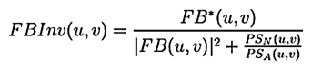
where FBInv is a fourier transform of inverse filter, FB^* is a complex conjugate of fourier transform of PSF, FB is fourier transform of PSF, PS_N is power spectrum of noise, PS_A is power spectrum of original image (can be substituted by power spectrum of observed image).

When we obtain FBInv the reconstructed image can be obtained as follows:

The inversion problem is formulated using a maximum a posteriori (MAP) approach which yields a functional that needs to be numerically minimized to obtain an estimate of the deconvolved object. This minimization is subject to physical constraints (e.g. nonnegativity of fluorescence intensities) and additional regularization constraints that encompass prior knowledge about the nature of typical fluorescence images (e.g. brightly shining objects on a dark background).

The convergence of the numerical algorithm is mathematically proven. This means that with suitable noise level settings, the results of the deconvolution will not diverge for an increasing number of iterations.

Articles concerning the algorithms were published by IEEE PAMI. Online access to the articles is charged and therefore cannot be shared here. Follow the links below to gain some more information.