Adjust Image

Background
Sharpen
ND Processing
Detect
Fourier Transform
Morphology
More Convolutions
Size
Convert
Rotate
Flip
Shift
Clear
Channel Alignment and Registration

Set the contrast degree by moving the first slider (1-100).
Set the radius by moving the second slider [µm].
Check the Preview check box to view the effect. If you are satisfied with the image, confirm the command by clicking .
Turn the Background ROI ON, or set any existing ROI as background (right-click a ROI and select Use as Background ROI).
Place the ROI so that it would define the background you would like to subtract.
Invoke the Subtract Background command. The average value of background is subtracted from each channel.
Light Background (Brightfield)
Black Background (Fluorescence)
Average Background (DIC, PhC)
Light Background (Brightfield) - for Brightfield
Black Background (Fluorescence) - for Fluorescence
Average Background (DIC, PhC) - for Differential Interference Contrast or Phase Contrast
Image intensity (signal is Bright)
Ball of the defined radius
Estimated background
It takes all frames of one Time layer (e.g. every first frame of all Z stacks).
It creates the Maximum Intensity Projection image from them.
It subtracts the maximum intensity projection image from every frame of the Time layer.
This procedure is performed on every Time layer of the current ND2 file.
It takes all frames of a Z stack.
It creates the Maximum Intensity Projection image from them.
It subtracts the maximum intensity projection image from every frame of the Z stack.
This procedure is performed on every Z stack of the current ND2 file.
It takes all frames of one Time layer (e.g. every first frame of all Z stacks).
It creates the Minimum Intensity Projection image from them.
It subtracts the minimum intensity projection image from every frame of the Time layer.
This procedure is performed on every Time layer of the current ND2 file.
It takes all frames of a Z stack.
It creates the Minimum Intensity Projection image from them.
It subtracts the minimum intensity projection image from every frame of the Z stack.
This procedure is performed on every Z stack of the current ND2 file.
It takes two subsequent frames of the Time loop - e.g. the first frames of the first (T1) and the second (T2) Z stack.
It subtracts the second one from the first one and saves absolute value of the result as the first frame:
Tresult = abs( T1 - T2 )All image pairs of all Time loop of the current ND2 file are processed.
It takes two subsequent frames of a Z stack - Z1 and Z2.
It subtracts the second one from the first one, and saves absolute value of the result as the first frame.
Zresult = abs( Z1 - Z2 )All image pairs of every Z stack of the current ND2 file are processed.
It takes two subsequent frames of the Time loop - e.g. the first frames of the first (T1) and the second (T2) Z stack.
It subtracts the second one from the first one, and saves the result as the first frame.
Tresult = T1 - T2All image pairs of all Time layers of the current ND2 file are processed.
It takes two subsequent frames of a Z stack - Z1 and Z2.
It subtracts the second one from the first one, and saves the result as the first frame.
Zresult = Z1 - Z2All image pairs of every Z stack of the current ND2 file are processed.
Brightfield - standard contrast based criterion
Fluorescence - suitable for fluorescence microscopy
Confocal - criterion based only on the intensity values. Can be useful in confocal microscopy.
Yeast, Bacteria (Ph) - a criterion optimized for yeasts under phase contrast (Ph) microscope.
Select the number of frames the average will be counted from.
Select the averaging method (Type).
Select the ND dimension to be averaged (Apply to).
Start the processing by clicking .
Run the Image > ND Processing > ND Images Arithmetics command. A window appears.
Select ND2 files from the top pull-down menus.
Select one of the available actions.
Check the preview and confirm it by OK. The operation will be performed on the corresponding image pairs.
 Addition = A+B
 Subtraction = A-B
 Absolute value of the difference = |A - B|
 Minimum = min(A,B)
 Maximum = max(A,B)
 Concatenate - this will connect the ND files one behind the other.
The Immunofluorescent Array tomography method - converting a multipoint to Z-Stack
Semi-automated Z-stack acquisition - when the user moves a Z-drive manually or via joystick while running the Acquire > Fast Time-lapse command. The resulting images are Time ND, but the user will convert them to Z-stacks.
Open an ND image.
Run the Image > ND Processing > Exchange Dimensions command.
Select one or more destination dimensions and adjust their properties.
It is important that the resulting ND file has equal or smaller number of frames than the original.
If you select more than one destination dimension, select the intended Experiment Order.
Select this command. The mouse cursor changes.
Click to draw a line in the image. Finalize it by a secondary mouse click outside the drawn line.
A new image called “Kymograph” is created.
Select whether to align to the Previous Frame (use for dramatic changes in the scene) or First Frame of the sequence (use for non-dramatic changes in the scene).
Select the size of the resulting ND2 file. If you prefer not to loose any image data, select The union of moved images.
Optionally, select:
Favor correction of the smooth movementFor time-lapse scenes containing slow and constant movement.
Process on the entire imageSuitable for stationary scenes where nothing moves.
Use correction for image heavily corrupted by noiseFor samples containing a lot of image noise.
Use SuperResolution aligmentFor high-precision alignment. However, this option slows down the processing and can slightly blur the resulting image.
Press . If the Process on the entire image is not selected, the procedure follows:
The mouse cursor changes waiting for you to draw a rectangle in the image. Draw the rectangle so it would contain some significant area such as a contrasting object. You can adjust its position and size by mouse.
Confirm the rectangle definition by the secondary mouse click. The application starts to align the ND2 file according to the selection.
Smooth
Vertical Edges
Horizontal Edges
Edges
None
Low
Medium
High
Create a user kernel (indicated by the human silhouette).
Define its size by editing the Size edit box. The denominator may be also edited.
Single values of the kernel can be edited after you clicked inside the appropriate cell, or the whole kernel may be inserted by the Paste from clipboard button.
Select the shifting units - voxels (in 3D), pixels (in 2D) or micrometers.
Define XY(Z) step size for the arrow and spin buttons.
Select a check box next to one channel to set it as reference. This channel will be always visible.
Note
Make sure the Synchronize View option is turned on.
Click a table row to give focus to the channel you want to shift (the row gets highlighted). Use the arrow buttons to shift the channel as necessary.
It is a good idea to open the ND image in another view (such as volume view) to check whether the shift between channels has been corrected.
Click to apply the shifts on all frames.
Open two ND2 files used for the alignment.
Run Image > Channel Alignment and Registration > Multimodal Image Registration.
Define which image is Fixed and which one is Moving.
Select a Merging strategy.
Click . Fixed image is placed on the left side, Moving is placed on the right.
Adjust the rotation/flipping of the Moving image if necessary.
Find at least one reference point contained in both images and mark it in both images using the
 Add Point tool. The more pairs of points you add the more precise the alignment will be.
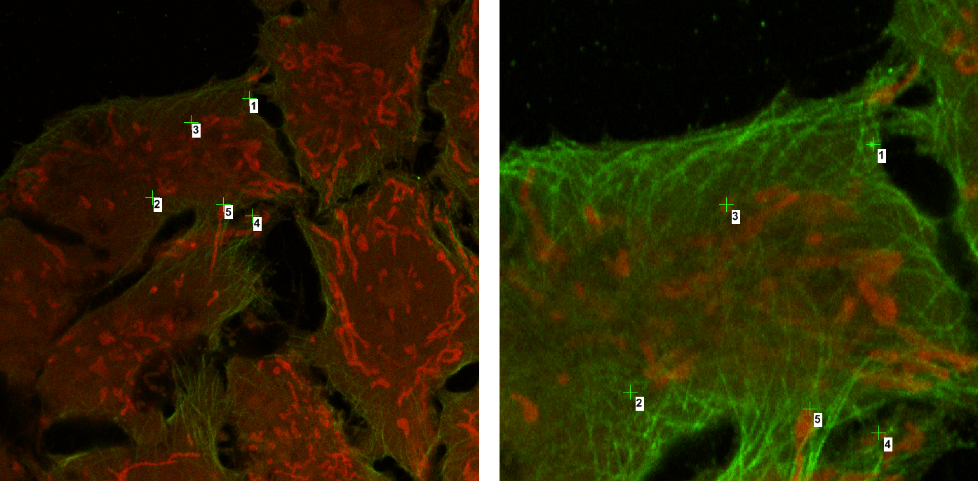
Figure 1799.
Click .
If the Save Registration Results dialog window appears, name your modalities and click so that the manual alignment does not have to be repeated for images captured by the similar hardware (see: Image > Channel Alignment and Registration > Optical Path Corrections).
New ND2 file with aligned images and merged attributes is created.
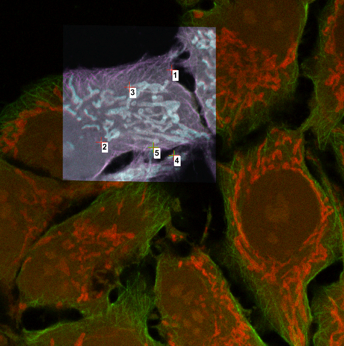
Figure 1800.
Select one of the predefined reference spectra listed in the Source Elements portion of the window.
Or, if any region of interest is defined, the image information from within a ROI can be used as reference spectra. Select the ROIs category, and select the actual ROI.
Or, the User Defined category is available, where arbitrary spectra definition can be loaded from a text file. This can be done within the Image > Manage Stored Spectra window.
Click the Add button to move the selected spectra to the Unmixing Elements table.

Increases contrast of the image. It changes intensities of the current image. Hue and saturation are not affected. Intensities are rescaled according to the selected method.
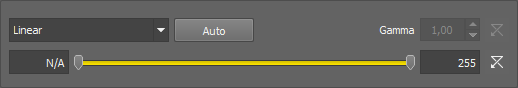
Figure 1720.
Options
Sets the Range so that the limits correspond to the minimum and maximum intensities found in the image.
The parameter for the Gamma Correction method. It ranges from 0.05 to 5.00. Set Gamma < 1 to get more information in dark areas or set Gamma > 1 to enhance bright parts of the image.
Set the low/high contrast intensities. Pixels with intensity greater than the high value set will be changed to a pure white, whereas pixels with intensity smaller than the low value set will be changed to pure black (zero). The range itself will be stretched to fit the available intensity range.
Closes the dialog window and applies the contrast settings.
Closes the dialog window without applying the contrast settings.
Opens this help page.
Turns the preview on/off.
See Image processing for description of other settings.
Methods
These transformations stretch the intensity interval defined by the range to the full intensity range using the selected curve. All values outside the range are set to pure black and pure white.
Equalization transformation leads to uniform intensity distribution in the specified interval <Low, High>.
Gamma correction maps the intensity interval <Low, High> according to exponential equation with the gamma parameter.
Enhances contrast of the current image while accentuating its details. The contrast is enhanced within both bright and dark areas of the image.
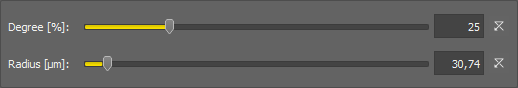
Figure 1721.
Procedure
Contrast multiplicator which is locally proportional to contrast amplification.
Size of the neighborhood to be processed.
Reset all dialog settings to default values.
See Image processing for description of other settings.
Enhances the contrast of each image component separately.
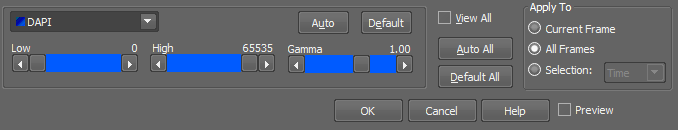
Figure 1722.
Selects component for processing: when you are processing an RGB image, press the button which corresponds to the desired channel. When processing a multichannel image, select which channel is used from the pull down menu.
Sets low intensity limit. Pixels with intensity less than Low will be set to zero.
Sets high intensity limit. Pixels with intensity greater than High will be set to 255.
Coefficient of gamma correction. Gamma correction maps the intensity interval <Low, High> according to exponential equation with parameter gamma. For gamma <1, you get the more sensitive information for the low intensities parts of image, whereas for gamma >1 higher intensities image parts are enhanced.
Performs automatic contrast enhancement.
Restores default values for Low, High and Gamma parameters.
If checked, all components (Red, Green, Blue or all multichannel components) of the image are displayed. If not checked, only the selected component is displayed.
Performs automatic contrast enhancement on all channels.
Restores default values for Low, High and Gamma parameters of all channels.
Apply the command to the whole image sequence, the selected dimension or just the current image frame. See ND2 Files Processing.
See Image processing for description of other settings.
Enhances details of the current image.
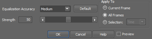
Figure 1723.
Choose the accuracy level of the image enhancement. The higher option you choose the more contrast is introduced into the final image.
Returns both Equalization Accuracy and Strength into their default values.
Defines the strength of the details enhancement. The higher value set the more details are accentuated and the more noise is introduced into the final image.
Apply the command to the whole image sequence, the selected dimension or just the current image frame. See ND2 Files Processing.
Balances and adjusts red, green and blue components of the current RGB image. One or two circular probes appear in the image. Move the probes to specify the white point and - optionally - the black point in the image.
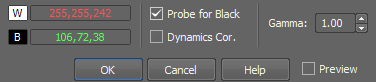
Figure 1724.
Shows Red, Green and Blue values for the white probe.
Shows Red, Green and Blue values for the black probe.
Shows the black level probe.
If checked, the values of all color components are recalculated to fit the full intensity range <0,255>.
Coefficient for gamma correction.
Note
Probe assignment is determined dynamically. If you move the red probe (white balance) over an image area which is darker then the area under the green probe (black balance), the probes swap automatically, so the text color in the window swaps as well to indicate the change.
See Image processing for description of other settings.
Transforms color image independently for each RGB component.
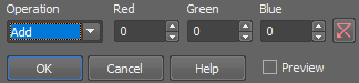
Figure 1725.
Type of image transformation.
Adds Red resp. Green resp. Blue value to red resp. green resp. blue component of each pixel.
Subtracts Red resp. Green resp. Blue value from red resp. green resp. blue component of each pixel.
Assigns minimum of red resp. green resp. blue component and Red resp. Green resp. Blue value to relevant component of each pixel.
Assigns maximum of red resp. green resp. blue component and Red resp. Green resp. Blue value to relevant component of each pixel.
Assigns Red resp. Green resp. Blue to red resp. green resp. blue component of each pixel.
Multiplies red resp. green resp. blue component of each pixel by Red resp. Green resp. Blue value.
Divides red resp. green resp. blue component of each pixel by Red resp. Green resp. Blue value.
Value used for red component.
Value used for green component.
Value used for blue component.
Initializes the previous value for selected color.
Apply the operation to the current image and close the window.
See Image processing for description of other settings.
Transforms intensities by arithmetic operations.
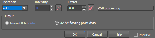
Figure 1726.
Type of the image transformation.
Adds Intensity to each pixel.
Subtracts Intensity from each pixel.
Selects minimum between each pixel intensity and Intensity.
Selects maximum between each pixel intensity and Intensity.
Sets the same Intensity to each pixel.
Multiplies each pixel by Intensity.
Divides each pixel by Intensity.
The value used for the arithmetic operation.
Value added to each pixel after the operation. It can be negative.
(requires: CA FRET) or
(requires: 2D Deconvolution) or
(requires: 3D Deconvolution)
Select data type of the output file. You can choose either the same original bit depth or 32-bit floating point image.
Note
Preview is disabled for 32-bit floating point data.
Displays the preview image.
Apply the operation to the current image and close the window.
See Image processing for description of other settings.
(requires: Dual Camera Support)(requires: Tripple/Quad camera support)
In some triple- or quad- camera configurations, you can turn on a speed optimization (by a registry key). It speeds up the acquisition but makes the captured image disordered. Use this command to repair such image to the standard format.

Changes saturation of an RGB image.
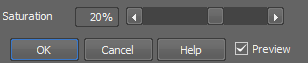
Figure 1727.
Expresses the degree of saturation enhancement. Positive values result in lively colors. Negative values de-saturate the image.
See Image processing for description of other settings.
Changes the color tone of an RGB image while maintaining its brightness and saturation.
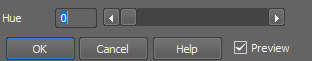
Figure 1728.
The hue is measured in degrees on the color wheel <0, 360>.
Apply the operation to the current image and close the window.
Note
This transformation is used for color image enhancement. Note, for instance, that positive hue shift turns blue color towards red.
See Image processing for description of other settings.
This command removes light parts of the image. Saturation of the image is increased.
See Image processing for description of other settings.
Mixes red, green and blue channels of the current RGB image arbitrarily.
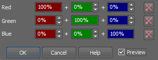
Figure 1729.
Each line defines the resulting color channel as a sum of percentages of all three channels. The sum is always 100%.
Apply the operation to the current image and close the window.
See Image processing for description of other settings.
Performs arithmetic division of intensities of two components of the current image. You can multiply the result and add a constant to it. The formula is clear from the dialog:
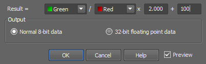
Figure 1730.
(requires: CA FRET) or (requires: 2D Deconvolution) or (requires: 3D Deconvolution)
Select data type of the output file. You can choose either the same original bit depth or 32-bit floating point image.
Select the box to preview the result.
Apply the operation to the current image and close the window.
Note
The function can be used to calculate the fraction of two selected image components, multiply and add offset to the result. Performing this command, the _DivideComponents is called.
See Image processing for description of other settings.
Adjusts the hue independently on each color channel of an RGB image.

Figure 1731.
Move the slider to change hue of the color channel.
Select it to display preview of the result.
See Image processing for description of other settings.

Transforms a color image into its complementary color image.
See Image processing for description of other settings.
This command provides an alternative to other noise reducing and details enhancing commands (Smooth, Sharpen, etc.). The procedure utilizes Fourier transformation. The following window appears.
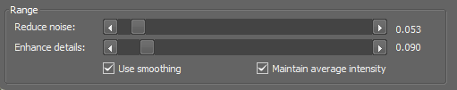
Figure 1732.
Check the Preview box in order to observe the influence of the transformation on the image.
Move the slider to set the level of reducing noise in the image.
Move the slider to set the level of details enhancement.
This check box regards the transformation procedure (it does not perform exactly smoothing on the image). If checked, the amount of image artifacts in the resulting image will be low.
Check this box in order to ensure the image to keep its original average intensity.
See Image processing for description of other settings.
This command subtracts background defined by the background probe from the whole image.
Subtracting background
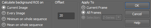
Figure 1733.
Choose how the background ROI is calculated.
Define custom value. The offset value adds a constant to the subtracted intensity, which is calculated as the average intensity of the background ROI, prior to subtraction in order to preserve image details.
See Image processing for description of other settings.
This command subtracts pixel values of the reference image from the current image. The reference image is created by the Reference > Current Image -> Reference menu command.
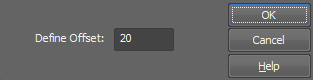
Figure 1734.
You can further modify pixel intensities of the corrected image by defining offset (positive or negative).
Subtracts a value from each channel separately.
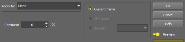
Figure 1735.
The value to be subtracted from each pixel of the selected channel. On RGB images, the value is subtracted from all channels automatically.
See Image processing for description of other settings.
This command defines parameters of the background shading correction.
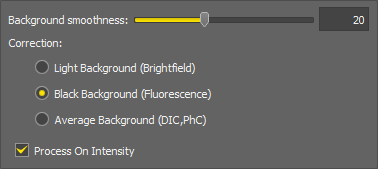
Figure 1736.
Defines the smoothness of the curve estimating the background. The lower the number the more smooth the curve is. With higher numbers the local changes become more accented.
Select on which background the correction is performed:
See ND2 Files Processing for description of common settings.
See also Acquire > Shading Correction Panel.
Performs the background shading correction only inside the ROI (Region Of Interest) area.
Select on which background the correction is performed:
Apply the command to the whole image sequence, the selected dimension or just the current image frame. See ND2 Files Processing.
Select this option to preview the effect of the operation on the current image.
See also Acquire > Shading Correction Panel.
Compensates image shading of the current image using a correction image specific for Confocal Microscope AX. The correction image is already a part of the function so no shading image needs to be acquired.
Move the slider to adjust how strong the correction effect will be.
Apply the command to the whole image sequence, the selected dimension or just the current image frame. See ND2 Files Processing.
Select this option to preview the effect of the operation on the current image.
See also Shading Correction
This function estimates the background intensity by rolling a ball of the defined radius over/under the image intensities.
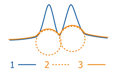
Figure 1737. Rolling Ball Background Correction Scheme
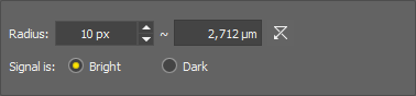
Figure 1738.
Set radius in pixels. The value should be bigger than size of the biggest object in the image.
Choose signal intensity - Bright for fluorescence images, Dark for bright-field images.
Apply the command to the whole image sequence, the selected dimension or just the current image frame. See ND2 Files Processing.
Select this option to preview the effect of the operation on the current image.

This command performs smoothing on the color image.
The Smooth Color Image dialog box appears:
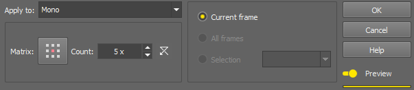
Figure 1739.
Click the button to change the structuring element used for this operation. See Matrix.
Number of iterations.
 Reset
Reset Sets the dialog default values.
Process each RGB channel separately or perform the processing on the intensity channel? See Image processing.
Select this option to preview the effect of the operation on the current image.
This function filters small irregularities in images.
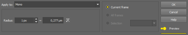
Figure 1740.
Select the size of neighborhood used for Median filtering.
Reset Sets the dialog default values.
Select this option to preview the effect of the operation on the current image.
See Image processing for description of other settings.
This function removes stripe patterns from the image.
Defines the strength of the stripe removing.
Reset Returns the strength value back to zero.
Select this option to preview the effect of the operation on the current image.
Performs the destripe processing.
Closes the window without applying the destriping processing.
Advanced denoising can be used to reduce any kind of noise in the image (Gaussian, Poisson noise). It can be applied on both 2D and 3D (Z-Stack) images.
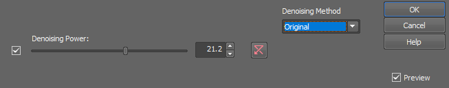
Figure 1741.
Define the strength of the denoising algorithm for each channel separately using the slider or the edit box. If the slider is set to zero, denoising is done with an estimated noise variance. Move the slider to the right and denoising calculates with higher noise variance (more noise is present in the image) and vice versa.
Choose a denoising method suitable for your image.
This method is based on denoising via pixel large neighborhoods in a spatial and frequency (incl. wavelets coefficients) meaning. It is a one-pass algorithm.
Iteratively denoises every pixel according to its local neigborhood. In every iteration, local linear regression is computed for every pixel and the value is replaced by the regressed value. This method belongs to the same family as the Original method.
Fusion between the Original and the Regression method. It takes the better parts of both algorithms.
This method is slower, but it uses a high-quality algorithm. A probabilistic approach is used to compute the most likely estimate from the neighboring pixels.
The method is very similar to the Regression method but in the new iteration, we find a new value by voting from extrapolation of neighboring pixels.
Select this option to preview the effect of the operation on the current image.
See ND2 Files Processing for description of common settings.
This command defines a filter, which passes only details larger than the set pixel value.
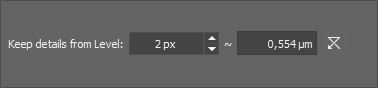
Figure 1742.
Set the size of details which will be kept. Smaller details will be suppressed.
Select this option to preview the effect of the operation on the current image.
Apply the command to the whole image sequence, the selected dimension or just the current image frame. See ND2 Files Processing.
Performs denoising of the current image captured by a resonant scanner. The algorithm was created using “deep learning” methods on a broad set of samples captured by a resonant/galvano scanner of Nikon A1. Therefore it is predetermined to give the best results when processing images from resonant scanners. A dialog window appears where the user selects channels to process.
This command enhances details of the image by creating a plastic-like imprint. Use this function in combination with LUTs to enhance barely visible details. Set the resolution degree using the slider.
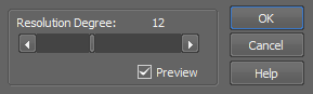
Figure 1743.
The lower the value the smaller details/objects get enhanced.
Select this option to preview the effect of the operation on the current image.
Apply the command to the whole image sequence, the selected dimension or just the current image frame. See ND2 Files Processing.

This function sharpens the image.
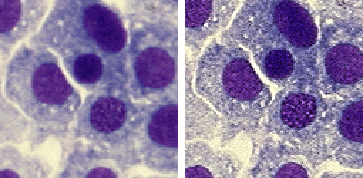
Figure 1744. Before - after applying the Sharpen function
See Image processing for description of other settings.
This function slightly sharpens the image.
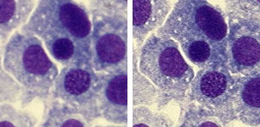
Figure 1745. Before - after applying the Sharpen Slightly function
See Image processing for description of other settings.
This command increases sharpness of the image. However, the scale in which the sharpening is performed is bigger than standard - i.e. large objects are affected, not tiny details.
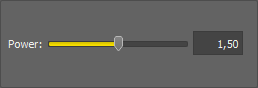
Figure 1746.
Set the power value. The possible range of values is from 1.01 to 2.
Sets the default value to the power text box. The default value is 1.25.
Select this option to preview the effect of the operation on the current image.
See Image processing for description of other settings.
Sharpens the image using the unsharp masking technique.
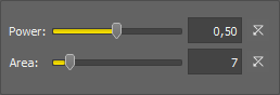
Figure 1747.
Set the strength of the sharpening effect. The possible range of values is from 0.01 to 1.
Define the area size which is used during calculating the result. The larger the area is, the smoother the result will be.
Sets the default value to the power text box. The default value is 0.5.
Select this option to preview the effect of the operation on the current image.
See Image processing for description of other settings.
It sharpens the image while suppressing countershading around edges often produced by unsharp masking. It is an improvement of the Image > Sharpen > Unsharp Mask function.
Set the strength of the sharpening effect. The possible range of values is from 0.01 to 1.
Define the area size which is used during calculating the result. The larger the area is, the smoother the result will be.
Sets Area and Power to default values.
Select this option to preview the effect of the operation on the current image.
See Image processing for description of other settings.
(requires: General Analysis)
This command enables applying General Analysis settings on captured images. For more details about General Analysis, please see the General Analysis chapter.
Recipes
Analysis settings can be saved as presets. These are called Recipes. Once done with adjusting the analysis parameters, you can save your recipe for later loading which can be done from the pull-down menu (Recipe database) or from a .ga file.
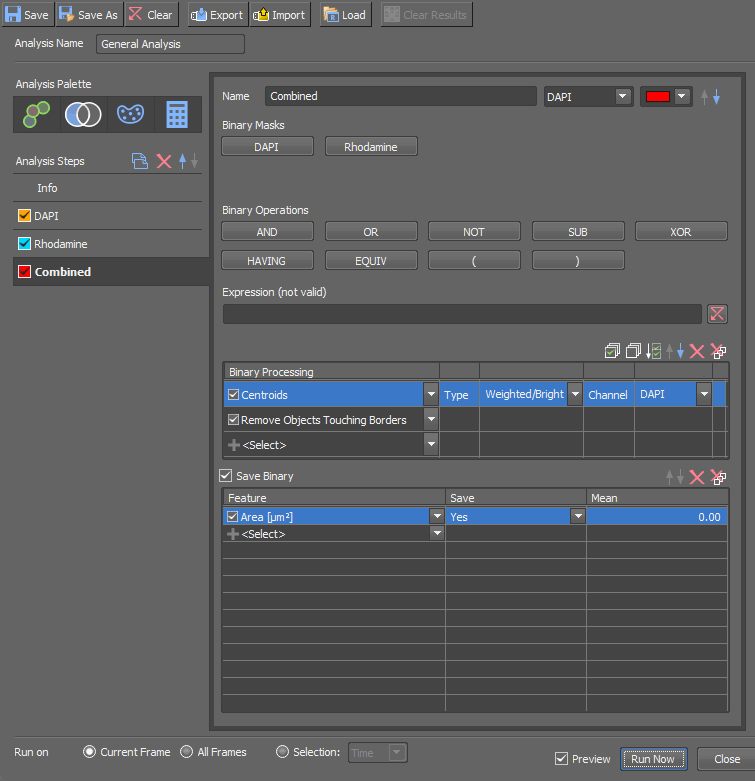
Figure 1748.
Main Toolbar
Loads a recipe from the recipe database. Choose <Manage...> to open the default folder containing recipe files.
Creates a new recipe with a given name.
Loads a previously saved recipe from a .ga file.
Saves any changes to the currently loaded recipe.
Saves a recipe as a file with a given name to any selected location.
This button clears all data shown in the View > Analysis Controls > Automated Measurement  tab which were captured by the current analysis.
Main Toolbar
 Save
Save Saves the current analysis settings into the database as a new recipe or updates any changes made to the currently used recipe. To load the recipe, use  Load.
Load.
 Save As
 Saves the current analysis settings into the database as a new recipe with a given name. To load the recipe, use Load.
Clear Resets the current analysis definition into default.
 Export
 Saves the current analysis recipe into an external *.ga file.
 Import
 Imports an analysis recipes from a *.ga file.
Load Opens the Load JOBS Recipe window enabling to select and import an analysis from jobs.
 Clear Results
 This button clears all data shown in the View > Analysis Controls > Automated Measurement tab which were captured by the current analysis.
(requires: General Analysis)
Displays the General Analysis RGB dialog window. It allows to create a new binary layer defined as an intersection of the three RGB channels based on the RGB or HSI threshold values. All other features of the dialog window are the same as in General Analysis (see: Image > General Analysis).
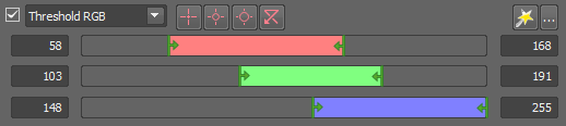
Figure 1749. RGB Threshold in General Analysis RGB
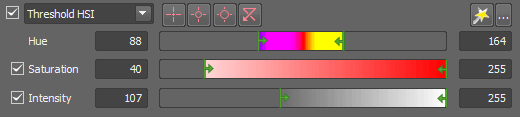
Figure 1750. HSI Threshold in General Analysis RGB
(requires: General Analysis)
Opens the latest version of the General Analysis 3. For more information please see General Analysis 3 .
(requires: General Analysis)
Opens the Batch GA3 dialog window used for running General Analysis 3 analyses in a batch order. Click on the button and select Content to open a help describing this function.
Analysis Explorer is closely described here: Analysis Explorer.
This command creates the maximum intensity projection image on the T dimension of the current ND2 document. Pixel values of the original image which have the same XY coordinates are compared throughout the image sequence and only the pixels with the highest intensity value are displayed in the new image.
This command creates the maximum intensity projection image on the Z dimension of the current ND2 document. Pixel values of the original image which have the same XY coordinates are compared throughout the image sequence and only the pixels with the highest intensity value are displayed in the new image.
This command creates the minimum intensity projection image on the T dimension of the current ND2 document. Pixel values of the original image which have the same XY coordinates are compared throughout the image sequence and only the pixels with the lowest intensity value are displayed in the new image.
This command creates the minimum intensity projection image on the Z dimension of the current ND2 document. Pixel values of the original image which have the same XY coordinates are compared throughout the image sequence and only the pixels with the lowest intensity value are displayed in the new image.
This command processes the Time dimension of an ND2 file in the following way:
This command processes all Z series of an ND2 file in the following way:
This command processes the Time dimension of an ND2 file in the following way:
This command processes all Z series of an ND2 file in the following way:
Calculates an average from the whole time sequence and subtracts it from each frame.
Calculates an average from the whole Z sequence and subtracts it from each Z plane.
This command processes the time dimension of an ND2 file in the following way:
This command processes all Z series of an ND2 file in the following way:
This command processes the time dimension of an ND2 file in the following way:
This command processes all Z series of an ND2 file in the following way:
This command creates a temporary “maximum intensity projection” image out of all frames of the current ND image and turns on the standard cropping tool. It prevents you from cutting off some important part of the scene just because it was not displayed in the current frame.
This command creates a temporary “minimum intensity projection” image out of all frames of the current ND image and turns on the standard cropping tool. It prevents you from cutting off some important part of the scene just because it was not displayed in the current frame.
This command enhances the dynamic range of generally any current ND2 file which contains at least time dimension. It analyses the image and calculates values similar to auto-contrast values common for the whole time sequence and then process all frames of the ND2 file. This method is robust to noise and preserves original trends of histogram.
You can select a method used to equalize the intensity.
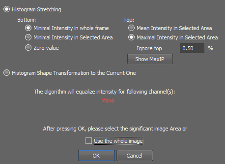
Figure 1751.
Select which method is used to equalize the document. The histogram is stretched using selected methods. The shape of the histogram is preserved.
This method transforms the shape of the histogram of the whole document according to shape of the histogram of the selected area.
After you press the OK button, you will be prompted to select according to which area the image will be equalized. Draw the rectangle and confirm with right-mouse click. The document is processed afterwards.
This command enhances the dynamic range of generally any current ND2 file which contains at least Z dimension. It analyses the image, calculates values similar to auto-contrast values common for the whole time sequence and then processes all frames of the ND2 file. This method is robust to noise and preserves original trends of histogram.
You can select a method used to equalize the intensity.
Figure 1752.
Select which method is used to equalize the document. The histogram is stretched using selected methods. The shape of the histogram is preserved.
This method transforms the shape of the histogram of the whole document according to shape of the histogram of the selected area.
After you press the OK button, you will be prompted to select according to which area the image will be equalized. Draw the rectangle and confirm with a right-mouse click. The document is processed afterwards.
This command adjusts intensities of image frames in different XY points of a multipoint ND document. It analyses the image and calculates values similar to auto-contrast values common for the whole multipoint sequence and then process all frames of the ND2 file. This method is robust to noise and preserves original trends of histogram.
You can select a method used to equalize the intensity.
Figure 1753.
Select which method is used to equalize the document. The histogram is stretched using selected methods. The shape of the histogram is preserved.
This method transforms the shape of the histogram of the whole document according to shape of the histogram of the selected area.
After you press the OK button, you will be prompted to select according to which area the image will be equalized. Draw the rectangle and confirm with right-mouse click. The document is processed afterwards.
This command automatically selects frames of an ND2 image sequence, the ones with the best focus. A new image is created.
Defines which focus criterion is used:
Choose which channels will be used when the best focus plane will be searched.
This command performs averaging on ND frames.
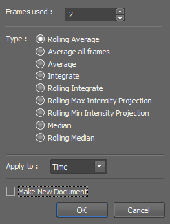
Figure 1754.
Choose the number of frames used for averaging.
This method takes the frames closest to the current frame, counts the average, and writes it to the current frame position. This method causes no loss of frames.
This method takes all frames, counts the average, and rewrites all frames. This option disables the Frames used option.
This method merges the adjacent frames, and counts the average. It reduces the number of frames in the ND2 file.
This method merges the adjacent frames, and adds them to each other. It reduces the number of frames in the ND2 file. The images get brighter.
This method integrates (sums) the adjacent frames. Number of adjacent frames can be set in the Frames used option. Number of frames of the result image is the same as in the original image. The images get brighter.
This method performs the Maximum Intensity Projection function on the defined number of frames. Number of frames of the result image is the same as in the original image.
This method performs the Minimum Intensity Projection function on the defined number of frames. Number of frames of the result image is the same as in the original image.
This method performs Median on the whole sequence (selected in the Apply to option). It reduces the number of frames in the ND2 file.
This method takes the frames closest to the current frame, performs Median, and writes it to the current frame position. Number of frames of the result image is the same as in the original image.
Select to which dimension will the averaging apply to. See ND2 Files Processing.
Result of this function is shown as a new document.
This command performs various operations on two ND2 files or on an ND2 file and an image. However, the documents must have a matching image resolution and the same dimensions structure.
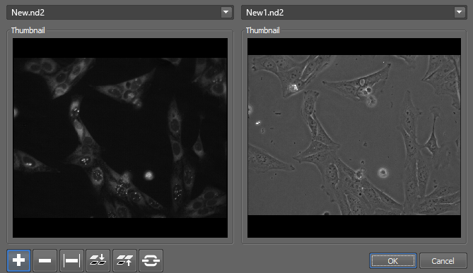
Figure 1755.
The processing can be performed using one ND2 file and a single image. Than, the operation is performed using the single image with each of the ND frames.
The following actions match certain mathematical operations. Let us call the ND2 files “A” and “B”.
This command converts a multi-frame 1DT (X or Y dimension + Time) image (created by Nikon A1 line-scan operation) to a single-frame 1DT image.
This commands can change structure of the current ND file. It does not process any image data so it is very fast.
Use cases
Usage
A kymograph gives a graphical representation of spatial position over time. In NIS-Elements, it displays pixel intensity changes under a defined linear section over time. A trajectory of a tracked object, or a user-drawn line can be used as the kymograph line.
See Also
Tracking
Line Thickness sets the size of the kymograph line. This line determines the neighborhood which is taken into account while using the Image > ND Processing > Create Kymograph by Line command. Intensity Computed As sets the intensity calculation method across lines thicker than 1 px. Pixel intensities of the resulting kymograph are calculated from the area covered by the line.
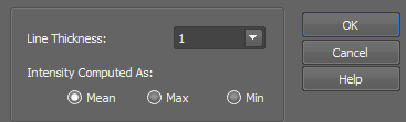
Figure 1756.
Note
Context menu over images having a T dimension reveals a quick option Create Kymograph By Line having the same functionality as Image > ND Processing > Create Kymograph by Line.
Line Thickness sets the size of the kymograph line. This line determines the neighborhood which is taken into account while using the Image > ND Processing > Create Kymograph by Line command. Intensity computed as sets the intensity calculation method across lines thicker than 1 px. Pixel intensities of the resulting kymograph are calculated from the area covered by the line.
Figure 1757.
Note
Context menu over images having a T dimension reveals a quick option Create Kymograph By Line having the same functionality as Image > ND Processing > Create Kymograph by Line.
This command aligns frames of an ND2 file. Depending on the type of your ND2 file, you will be prompt to select the dimension to which the alignment will be applied. After that, a dialog window appears:
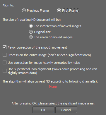
Figure 1758.
Note
Precision of the resulting alignment depends on image quality and therefore can not be guaranteed. If the result is not satisfactory, please use manual means to align the ND image. See Shifting Image Channels, Image > Shift > Right, Image > Shift > Left, Image > Shift > Up, Image > Shift > Down
This command converts a multi-point ND2 file into a large image. The XY coordinates contained in the multi-point dimension are used to arrange the images correctly. If the original scanned area was not homogeneous, the blank places will be filled with a background color.
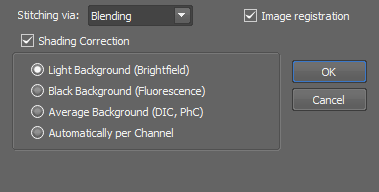
Figure 1759.
Options
Select how image margins will be treated:
Overlapping image parts will be blended.
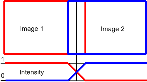
Figure 1760. Stitching via "Blending" (pixel intensity is changed in the overlapped region)
A contour where two overlapping images are least different will be computed. The images will be stitched copying this contour.
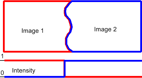
Figure 1761. Stitching via "Optimal path" (pixel intensity is preserved)
Position of images can be adjusted automatically based on texture comparison. If there are pixel-shifts between neighboring images, this function will help.
Select whether to perform the shading correction and which type of image you are stitching (type of the image background). If Automatically per Channel is selected, the shading modality method is detected and applied per channel.
Please see Acquire > Shading Correction Panel.
This command converts opened ND2 file created by Custom Acquisition to Time-lapse format.
For more details about Custom Acquisition see Acquire > Custom Acquisition.
This command converts opened ND2 file created by Custom Acquisition to ZStack format.
For more details about Custom Acquisition see Acquire > Custom Acquisition.
This command converts opened ND2 file created by Custom Acquisition to Multipoint format.
For more details about Custom Acquisition see Acquire > Custom Acquisition.
This command enables advanced operations with images.
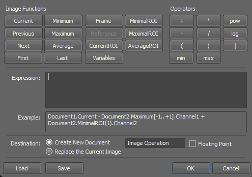
Figure 1762.
Press the button of a corresponding function from the variety of available functions to insert it to the custom equation.
Uses the current frame intensity of the opened document and its channel(s).
Uses the previous frame intensity of the one opened document and its channel(s).
Uses the next frame intensity of the one opened document and its channel(s).
Returns the first image or channel in a sequence.
Finds minimal frame(s) intensity of the one opened document and its channel(s).
Finds maximal frame(s) intensity of the one opened document and its channel(s).
Finds average frame(s) intensity of the one opened document and its channel(s).
Returns the first image or channel in a sequence.
Uses the selected frame intensity of the one opened document and its channel(s)
Uses the Reference Image intensity.
Uses the current ROI intensity.
A list of system variables appears and you can select one to be used in the expression.
Finds the minimal ROI intensity.
Finds the maximal ROI intensity.
Finds the average ROI intensity.
Define further parameters of the selected function in the dialogs that appear after you press the corresponding button:
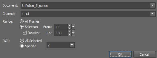
Figure 1763. Example of selection of possible parameters
Choose which document is processed.
Choose which channel is processed.
Define range of processed frames of an ND document: All Frames, or Selection (From, To) can be selected. If you check the Relative option, the range can be defined relatively. Then the current frame's number is 0, previous frames are defined by negative numbers and next frames by positive numbers.
Define which ROIs are processed.
Define index of a frame to be processed by the function. If you check the Relative option, the index can be defined relatively.
Press the button of a corresponding operator to insert it to the custom equation.
Operators
Addition
Subtraction
Multiplication
Left bracket
Right bracket
Absolute value
Division (requires: CA FRET) or (requires: 2D Deconvolution) or (requires: 3D Deconvolution)
Minimum of two or more values
Maximum of two or more values
Power function (requires: CA FRET) or (requires: 2D Deconvolution) or (requires: 3D Deconvolution)
Logarithm function (requires: CA FRET) or (requires: 2D Deconvolution) or (requires: 3D Deconvolution)
Write the custom expression into this field. Use the functions and operators provided in the window. You can also edit the expression manually.
Select what to do with the resulting image. If you choose the Create New Document option, you can edit name of the new file in the edit box.
There is also a possibility to create the floating point image as the result of operation. (requires: CA FRET), (requires: 2D Deconvolution) or (requires: 3D Deconvolution)
Loads previously saved settings from an external file.
Saves current settings to an external file.
Opens the Radon Transform dialog window applying the Radon Transformation (see Radon Transform).
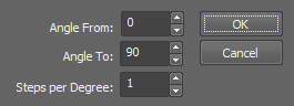
Figure 1764.
Low angle value [°].
High angle value [°].
Number of steps per one degree.
Apply the command to the whole image sequence, the selected dimension or just the current image frame. See ND2 Files Processing.

Detects edges by morphological transformations on color images.
The DetectValleys dialog box appears:
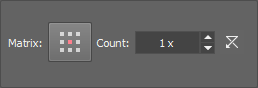
Figure 1765.
Click the button to change the structuring element used for this operation. See Matrix.
Number of iterations.
Reset Sets the dialog default values.
Apply the operation to the current image and close the window.
Process each RGB channel separately or perform the processing on the intensity channel? See Image processing.
Apply the command to the whole image sequence, the selected dimension or just the current image frame. See ND2 Files Processing.
Note
The Detect Valleys command enhances small dark objects by “Top Hat” morphologic transformation. The size of the selected objects is determined by level of the transformation, which depends on Matrix type and on Number of steps. This command enables the specific segmentation of small objects to the exclusion of larger objects and also can help you in the case of non-homogeneous background.
The Detect Valleys (Top Hat) dialog box appears.
Figure 1766.
Click the button to change the structuring element used for this operation. See Matrix.
Number of iterations.
Reset Sets the dialog default values.
Apply the operation to the current image and close the window.
Process each RGB channel separately or perform the processing on the intensity channel? See Image processing.
Apply the command to the whole image sequence, the selected dimension or just the current image frame. See ND2 Files Processing.
Note
Detect Peaks command enhances small light objects by “Top Hat” morphologic transformation. The size of objects selected is determined by the size of the used structuring element, which depends both on Matrix and Number parameters. This command enables the specific segmentation of small objects to the exclusion of larger objects and also can help you in the case of non-homogeneous background.
The Regional Minima function detects regional minima. It is a subset of top hat transformations.
The Regional Minima dialog box appears.
Figure 1767.
Click the button to change the structuring element used for this operation. See Matrix.
Number of iterations.
Reset Sets the dialog default values.
Apply the operation to the current image and close the window.
See Image processing for description of other settings.
Detects regional maxima. It is a subset of top hat transformations.
The Regional Maxima dialog box appears.
Figure 1768.
Click the button to change the structuring element used for this operation. See Matrix.
Number of iterations.
Reset Sets the dialog default values.
Apply the operation to the current image and close the window.
See Image processing for description of other settings.
This command enhances the edges in the image.
See Image processing for description of other settings.
Detects edges by morphological transformations of color images.
The Morphologic Gradient dialog box appears:
Figure 1769.
Click the button to change the structuring element used for this operation. See Matrix.
Number of iterations.
Reset Sets the dialog default values.
Process each RGB channel separately or perform the processing on the intensity channel? See Image processing.
Apply the command to the whole image sequence, the selected dimension or just the current image frame. See ND2 Files Processing.
Note
Morphologic gradient is the difference between dilated and eroded images. It enhances edges.
This command can enhance objects in a DIC image so that the objects can be thresholded reasonably.
The Differential interference contrast capturing method produces special kind of images, where objects look three-dimensionally having glow on one side and shadow on the other side. Such objects can not be thresholded and further analysed. The Detect DIC Objects command performs recognition of the objects and makes them bright in order to be easily thresholded.
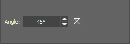
Figure 1770. Detect DIC Objects dialog for Multichannel images
Specify the angle of illumination in the edit box.
Select this option to preview the effect of the operation on the current image.
Apply the command to the whole image sequence, the selected dimension or just the current image frame. See ND2 Files Processing.
See Image processing for description of other settings.
Gabor Edge Detection method represents a linear filter useful for visualizing specific features of an image. Use the Orientation combo box to select a direction [°] in which the features are visualized. Select a proper direction and adjust the Amplitude of the wavelet to find the sharpest result. Real, Imaginary or Both filters can be applied. Switching from Positive to Negative Value highlights the surroundings of the object.
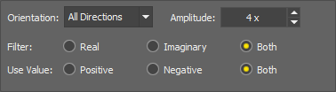
Figure 1771.
Select a direction in degrees in which the features are visualized.
Adjust the amplitude of the wavelet to find the sharpest result.
Apply one of the filters or both.
Switching from Positive to Negative highlights the surroundings of the object.
Detects edges of objects based on the Rolling Ball Radius value and Light/Dark signal using the Canny algorithm.
Start by setting the level of details (Edge Size) and then define the Low and High threshold value to include/exclude targeted portions of your image. Check the Preview check box to see the result. Once you are satisfied with the detection, click to apply it to your image.
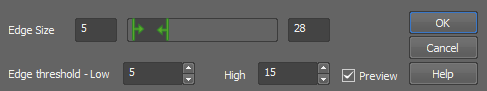
Figure 1772.
Serves to recover a function from its Fourier transformation.
Applies binary mask on the Fourier transform image.
Opens the Log Power Spectrum dialog window applying the 2D Fourier Transformation (see Fourier Transform).
Performs morphological opening on current color image. Morphological opening is erosion followed by the same number of dilations. The transformation removes small light objects. If the structuring element dimension has an odd value, there are two enhanced pixels in structuring element depicting centers: one for erosion and the other for dilation.
The Open Color Image dialog box appears.
Figure 1773.
Click the button to change the structuring element used for this operation. See Matrix.
Number of iterations.
Reset Sets the dialog default values.
See Image processing for description of other settings.
Performs morphological closing on the current color image.
The Close on Color Image dialog box appears.
Figure 1774.
Click the button to change the structuring element used for this operation. See Matrix.
Number of iterations.
Reset Sets the dialog default values.
See Image processing for description of other settings.
Morphological closing is a dilation followed by the same number of erosions. Small dark areas are removed by this transformation. If the structuring element dimension has an odd value, there are two enhanced pixels in structuring element depicting centers: one for erosion and the other for dilation.
Performs morphologic erosion on color image. Erosion affects the intensity of color image. Hue and saturation are not affected. Dark areas grow whereas light areas shrink.
The Erode Color Image dialog box appears.
Figure 1775.
Click the button to change the structuring element used for this operation. See Matrix.
Number of iterations.
Reset Sets the dialog default values.
Apply the operation to the current image and close the window.
See Image processing for description of other settings.
See Also
Image > Morphology > Open Image > Morphology > Open, Image > Morphology > Close Image > Morphology > Close, Image > Morphology > Dilate, Image > Morphology > Linear Erode
Performs morphological dilation on color image. Dilation of color images changes their intensity. Light areas grow and small dark objects and structures disappear. Hue and saturation are not affected.
The Dilate Color Image dialog box appears.
Figure 1776.
Click the button to change the structuring element used for this operation. See Matrix.
Number of iterations.
Reset Sets the dialog default values.
Apply the operation to the current image and close the window.
See Image processing for description of other settings.
Removes small light areas in the direction specified by Matrix.
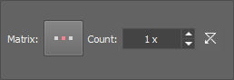
Figure 1777.
Click the button to change the structuring element used for this operation. See Matrix.
Number of iterations.
Reset Sets the dialog default values.
Apply the operation to the current image and close the window.
See Image processing for description of other settings.
Closes color image using a linear structuring element.
The Linear Close Color Image dialog box appears.
Figure 1778.
Click the button to change the structuring element used for this operation. See Matrix.
Number of iterations.
Reset Sets the dialog default values.
Apply the operation to the current image and close the window.
Note
Linear morphological closing is a dilation followed by erosion using the same linear structural element. The transformation is performed on the intensity component and removes small dark areas in the direction specified by Matrix orientation. Number specifies level of closing.
See Image processing for description of other settings.
Erodes color image using a linear structuring element.
The Linear Erode Color Image dialog box appears.
Figure 1779.
Click the button to change the structuring element used for this operation. See Matrix.
Number of iterations.
Reset Sets the dialog default values.
Apply the operation to the current image and close the window.
Note
Linear erosion affects the intensity of color image in one direction. Hue and saturation are not affected. Dark areas linearly grow whereas light areas linearly shrink in the direction defined by Matrix orientation. It is an anisotropic transformation.
See Image processing for description of other settings.
Erodes color image using a linear structuring element.
The Linear Dilate Color Image dialog box appears.
Figure 1780.
Click the button to change the structuring element used for this operation. See Matrix.
Number of iterations.
Reset Sets the dialog default values.
Apply the operation to the current image and close the window.
Note
Linear dilation of color images changes their intensity in one direction, specified by Matrix orientation. Light areas linearly grow and small linear dark objects and structures disappear. Hue and saturation are not affected. It is an anisotropic operation.
See Image processing for description of other settings.
This function performs edge detection by Laplace4 detector.
See Image processing for description of other settings.
This function performs edge detection by Laplace8 detector.
See Image processing for description of other settings.
This function sharpens the image.
Figure 1781. Before - after applying the Sharpen More function
See Image processing for description of other settings.
This function performs horizontal edge detection.
See Image processing for description of other settings.
This function performs vertical edge detection.
See Image processing for description of other settings.
This function performs filtration on intensity component (or on every selected component - when working with multichannel images) of an image using convolution with 5x5 kernel. Mexican Hat kernel is defined as a combination of Laplacian kernel and Gaussian kernel, it marks edges and also reduce some noise.
See Image processing for description of other settings.
Smooths and detects edges of color image.
The Golay filter dialog box appears.
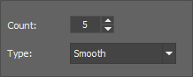
Figure 1782.
Number of steps used in the algorithm.
Type of filter.
Note
Golay filter function uses polynomial (second order) fitting of the image data for smoothing image. Fitting is performed in the neighborhood defined by Kernel parameter. The Vertical Edges detection is derived from the 1st derivation of image data in the X direction. The same is true for Horizontal Edges detection (Y direction). General edge detection is calculated as the sum of the absolute values of the 1st derivations in X and Y directions. Edge detection includes dynamics corrections. Algorithm exactly calculates edge values.
See Image processing for description of other settings.
Enhances edges and smooths homogeneous areas in color image. The Delineate dialog box appears:
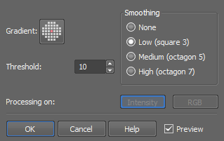
Figure 1783.
Size of matrix for gradient detection.
Size of matrix for smoothing.
Threshold value for gradient.
Apply the operation to the current image and close the window.
Process each RGB channel separately or perform the processing on the intensity channel? See Image processing.
Apply the command to the whole image sequence, the selected dimension or just the current image frame. See ND2 Files Processing.
Note
In the resulting image, edges are enhanced and smooth areas are more homogeneous.
Creates a pseudo 3-D image. The Relief dialog box appears:
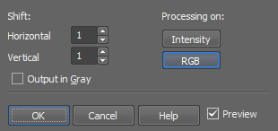
Figure 1784.
Sets the shift (in pixels) along X axis.
Sets the shift (in pixels) along Y axis.
If checked, the result of the transformation is a gray image. This option is only applicable to RGB images.
Process each RGB channel separately or perform the processing on the intensity channel? See Image processing.
Apply the command to the whole image sequence, the selected dimension or just the current image frame. See ND2 Files Processing.
Note
Superimposition of the original and the shifted image results in a pseudo 3-D image.
This command is used for creating new or modifying the existing convolution kernels and applying the convolution to an image.
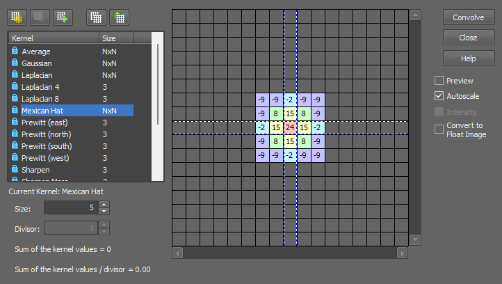
Figure 1785.
There is a list of predefined (locked) kernels which can be extended by kernels of your own. Use the following buttons:
 New
New This button creates a new empty kernel.
 Delete
 Deletes the selected user kernel. Predefined kernels cannot be deleted.
 Copy current
 This button creates a copy of a selected kernel.
 Copy to clipboard
 Copies the kernel to memory as tab delimited values. The kernel may be inserted to a spread sheet editor or a text file.
 Paste from clipboard
 Inserts the tab delimited values from clipboard as a new user kernel. Arbitrary user kernel can be created in an external application, copied, and inserted by this button.
Modifying kernel
Convolution Options
Select this option to preview the effect of the operation on the current image.
Usage of some kernels may result in pixel values which it is impossible to display within the image (negative values, high values). Such values would be clipped to fit the acceptable range (0-255 for 8bit images), and you could loose certain amount of image information because such pixels would turn black/white. However, you can prevent this image distortion by using the Autoscale option. It maps all the computed values to the acceptable range so it can be displayed correctly.
You can decide whether to perform the convolution channel by channel, or on the intensity only. This option is only applicable for RGB images.
Floating point images are supported. If the provided image is an integer and this option is checked, the image will be converted to a floating point image.
See Image processing for description of other settings.

Cuts off everything outside the selected area. Selecting this command invokes the crop cursor. Click the primary mouse button and drag to define the cropping area. Adjust the area you want to crop using the red rectangle. Move the white squares on the rectangle edges to adjust its size and move the whole rectangle using the primary mouse button to set its position.
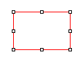
Figure 1786. Cropping rectangle
Another way to set the crop is to use the dialog window in which you can specify the Left and Top corners of the rectangle, its Width, Height and the units used (pixels, µm, mm). Once you finish defining the cropping rectangle, confirm it by clicking .
The Draw Rectangle... button hides the dialog window and lets you draw the cropping rectangle manually. Remember Last Settings remembers the crop data which can be reused in future image cropping. If the image being cropped with the remembered data is smaller than the previously cropped one, it may be reduced and moved automatically.
Splits an image into separate tiles. Please see Splitting Large Images for more information.
Using this command it is possible to adjust image dimensions. You can enter the new size as an exact value in pixels or in percents of the current image.
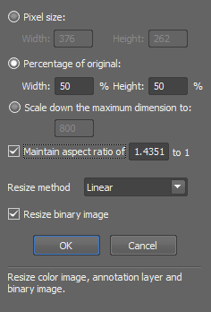
Figure 1787.
If this option is chosen, you need to enter new dimensions of the image in pixels.
In case this option is checked, you can enter the size of new image in percents of the current image.
Scales down the image. The longer side of the image is rescaled to the defined number of pixels while the aspect ratio is kept. Shorter side of the image is calculated automatically.
If this option is active, you can enter only one dimension of new image and the other is filled automatically to keep selected aspect ratio. Aspect ratio is computed and prefilled according to your current image dimensions.
You can choose from three different resize algorithms. Try which one works best for your application.
Every NIS-Elements image consist of three (or more) layers (Color, Binary, Annotation...). The Color and annotation layers are linked together, but binary image behaves independently. Checking this option causes simultaneous resizing of both Color and Binary layers.
See Also
Image > Convert > Change Color Depth
This command sets the dimensions of current image. Selecting this command displays the following window:
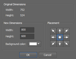
Figure 1788.
The upper part of window is informational and shows current image dimensions. You can set new dimensions using the Width and Height edit-boxes. The image will not be resized, but cropped (in case of new dimensions are smaller than the old ones) or placed in the image, surrounded by borders in background color (in the case of new dimensions are grater than original image). You can define the placement of an old image in the new image using the arrow button tool.
This command adds color borders to current image. Selecting this command, the following dialog box appears:
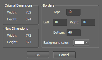
Figure 1789.
The left side of window is dedicated to information about image size. The original dimensions are displayed here.
You see the dimensions with borders added.
Four-edit boxes on the right serve for entering the border thickness in pixels. Each edit-box stands for one image side. The color of image frame is possible to define using color picker called Background color.
Opens the Image Binning dialog window enabling to bin the current image based on the binning factor and binning method.
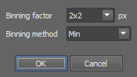
Figure 1790.
Binning factor of 3x3 will reduce the area of 9 pixels into a single pixel in the resulting image based on the selected method.
The resulting pixel value will be calculated as maximum, minimum, mean or sum. Sum No Noise - this method brightens the image but does not amplify noise like the Sum method does.

Transforms current color image into gray image. The resulting intensities are defined for every pixel as an average of red, green and blue component values.
When you are analyzing a ND2 file, select the frames to which the function is applied in the window that appears.
Transforms the current gray image into a color image. The resulting RGB image consist of three components with identical values. The image looks still grey.
This command changes the image (image) type of the current RGB image to Multichannel. The Custom channel is appended.
Converts color image from standard RGB representation to HSI representation. The standard RGB color image representation is natural for NIS-Elements G and the image is displayed in its original colors on the monitor. The HSI image cannot be displayed in its original colors.
Converts color image from HSI representation to standard RGB representation. The HSI color image is transformed to RGB representation. It is the inverse function to Convert RGB to HSI; after these transformations the image retains its original colors.
Converts current binary image to color image. The content of image remains unchanged but the image obtains color status. In another words, objects in binary image are transformed to areas with white color (RGB=(255, 255, 255)) in current color image. Background in current binary image is transformed to black (RGB=(0,0,0)) in current color image. This means, that all color transformations commands become available.
This command appends the contents of the active (visible) binary layer to the current image as a new channel. The original color of the binary layer is used for the channel. If multiple binaries are visible, one channel will be created for each binary layer.
Note
In case of a multi-frame image, the function is applied to all frames automatically.
This command changes the color depth of the current image. You can increase or decrease the depth to 8, 10, 12 or 16 bits.
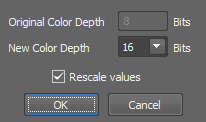
Figure 1791.
Displays the color depth of the current image.
Sets a new color depth of your image. You can choose from 8, 10, 12, 16 bit.
If checked the pixel values are mapped to the new range. E.g. when you convert an 8bit image to 16bit and you do not select to rescale values, it results in a completely black image. If the check box was selected, the 8bit 255 value would become 65535 in 16bit etc.
See Also
Image > Size > Resize
Use this command to convert a floating point image to a new standard image. Define which method is used to convert the currently opened floating point image to integer values. Select the bit depth of the new image. Recommended bit depth is displayed below the pull down menu.
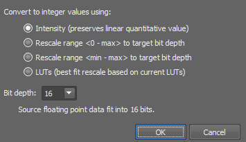
Figure 1792.
Converts the image to integer values with minimum loss of quantitative information.
Stretches the interval “0 to image maximimum” to fit the target bit depth.
Stretches the interval “image minimum to image maximimum” to fit the target bit depth.
Stretches the interval “LUTs black slider to LUTs white slider” to fit the target bit depth. See LUTs - Non-destructive Image Enhancement.
Select target bit depth of the resulting image.
(requires: CA FRET)
This command converts current image to new floating point image.
Transforms an RGB image to one of its RGB or HSI components. On multichannel images, the HSI color space is not available.
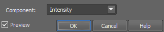
Figure 1793.
Select the type of component to be extracted from the pull down menu.
A channel from the RGB color representation.
A component from the HSI color representation. Not available
Note
In the resulting gray image all RGB components are identical and the image is stored in the same way as a “usual” color image.
Adds a new channel to the current image. The following dialog appears:
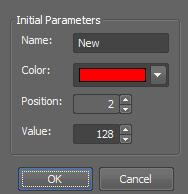
Figure 1794.
Enter a name of the new channel.
Select its color from the color palette.
Set its position within the existing channel.
Set the intensity of all pixels of the new channel.
Performs free image rotation. The Rotation dialog box appears:
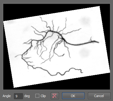
Figure 1795.
Defines the angle of the rotation. The rotated image is previewed in the dialog box. The angle is oriented with value ranges from 360 to -360 degree.
Crops the rotated image
Reset Sets the rotation angle back to 0 degree.
Performs a rotation via line. Drawing the line you specify only the angle of rotation. The center of the rotation will be in the center of the image. Defined line in the image is rotated to become horizontal using the sharp angle. Rotated image is computed from the source using 4-neighbourhood.
Performs rotation via line. Line in the image is rotated to become horizontal. Drawing the line you specify the center and the angle of rotation. Defined line in the image is rotated to become horizontal using the sharp angle. Rotated image is computed from the source using 4-neighbourhood.
Performs rotation via line. Line in the image is rotated to become vertical. Drawing the line you specify the center and the angle of rotation. Defined line in the image is rotated to become vertical using the sharp angle. Rotated image is computed from the source using 4-neighbourhood.
Enables you to select a rectangular shaped part of an image and adjust its final orientation. The rest of the image will be cut off.
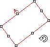
Figure 1796.
Place, resize and rotate the red rectangle. When you confirm the action by right click, the command will crop the image and rotate the selected area, so that the red arrow will point upwards.
This command moves the current image or a selected component by one pixel in the defined direction. The pixels that overflow the image borders appear on its opposite side.
When using this command via the key shortcut (Ctrl+Shift+Arrow) on a single component, all components are displayed together until the Ctrl+Shift keys are released.

This function clears the color layer of a image. All pixel intensities are set to zero.
Clears current annotation layer and sets color of all pixels to transparent.
Opens the Align Channels dialog window enabling to manually shift each channel in the X, Y or Z direction.
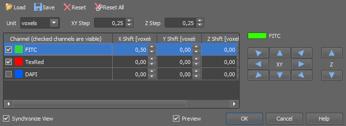
Figure 1797.
Example procedure
Dialog Window Options
 Load
Load Load previously saved shift settings from the list.
Save Use this button to save shift settings for later use.
 Reset
Reset Clears shift settings of the selected (highlighted) channel.
 Reset All
 Clears shift settings for all channels.
Voxels (3D), pixels (2D), micrometers for calibrated images.
Step used by the arrow buttons. Uses the selected units.
If turned on, only channels selected in the table (checked or highlighted) are displayed. Deselect the option to control the display by channel tabs in the image window.
Corrects the image color shifts. Color shifts most likely origin when you are using two cameras for capturing one scene. The cameras can have different resolution or are not aligned properly. So when you put the two grabbed images together, they do not match each other perfectly.
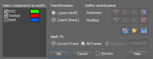
Figure 1798.
Check the component(s) you want to modify. The unchecked component(s) remain unchanged.
Select the way how to match the components.
This option allows to shift the components. You have to define one point.
This option allows to fit the components more precisely, but it changes the calibration of the modified components. The modified components are shifted, rotated and stretched to fit the stationary components. The definition is done by setting three point.
Use the button to define one or three control points (depending on the selected method). Press the Stationary point button and click into the image to mark the stationary point. Then place the Modified point mark. Then define the remaining two points (for 3-point method). To see each component (stationary/modified) separately during control point definition, press the  button. To reset all definitions, press the button.
The  Fine Tune button runs an algorithm that tries to correct small differences in point definition using alignment in near neighborhood of defined point. It does not invoke any action but it keeps the state and have influence on automatic alignment done after all points are defined.
See ND2 Files Processing.
See ND2 Files Processing.
Opens the Registration Wizard dialog window which can be used to manually align two images and create a new ND2 document combining both perfectly aligned images.
Typical alignment procedure
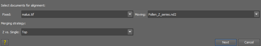
Figure 1801.
Documents for alignment
Defines the fixed image from which the FOV is taken. The resulting aligned image will have the same FOV as this image. The highest possible resolution from both image pairs is maintained. This image will be placed on the left side after clicking .
Defines the image which will be positioned over the Fixed image. This image will be placed on the right side after clicking .
Merging strategy
Z stack in the left image often has a different amount of planes than in the right image. Merging strategy defines how the missing planes are obtained. Any undefined planes will be shown black in the resulting image.
Single Z plane is placed at the top of the Z-stack.
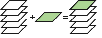
Figure 1802. Z - Single: Top
Single Z plane is placed at the bottom of the Z-stack.
Figure 1803. Z - Single: Bottom
Single Z plane is placed over the home position of the Z-stack.
Figure 1804. Z - Single: Home
Single Z plane is placed over the whole Z-stack.
Figure 1805. Z - Single: Duplicate
Single Z plane is placed over the closest Z-plane based on the Z distance obtained from Recorded Data.
Figure 1806. Z - Single: Closest Z
Planes with Z distance closest to the Fixed image are taken into account. Left Fixed image is used as a reference image from which the Z-step is taken. Planes lying in the Z distance range of the Z-step are included in the result whereas others are displayed black.
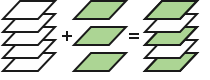
Figure 1807. Z - Z: According to Z
Missing planes are linearly interpolated across the Z-distance between two adjacent planes.
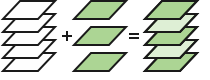
Figure 1808. Z - Z: Interpolated
If the Moving image is a single frame, this option places it over the first frame of the resulting time lapse.
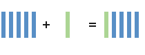
Figure 1809. T - Single: First
If the Moving image is a single frame, this option places the image over all frames of the resulting time lapse.
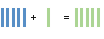
Figure 1810. T - Single: Duplicate
Note
Matching two time lapse images is not supported and multi-point images cannot be included in the alignment.
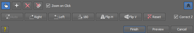
Figure 1811.
Dialog Window Options
 Hand tool
 Standard hand tool used to move inside a zoomed image.
Add point Adds an alignment point by clicking into the Fixed or Moving image.
Delete point Deletes a point on a mouse click.
Delete all points Deletes all points.
Check the check box, left-click into the image and hold the mouse button to zoom into the clicked area, position the mouse and release the button to place an alignment point.
 More Options
 Displays tools for rotating and flipping the Moving image.
 Auto
Auto Rotates the image according to information taken from image metadata. If registration results are available, they are automatically applied.
 Right
Right Rotates the Moving image by 90° right.
 Left
Left Rotates the Moving image by 90° left.
 180°
180° Rotates the Moving image by 180°.
 Flip Horizontally
 Flips the Moving image horizontally.
 Flip Vertically
 Flips the Moving image vertically.
Reset Removes any alignment and rotation made by registration results, turns off the Auto function and zooms the Moving image to  Best Fit (View > Zoom > Best Fit ).
If the two Z stack images opened for alignment were captured using different objectives, it is almost certain that the Z distance is shifted. Use this function to correct the shift. Z distance of the Moving image is automatically corrected by the difference of Z positions of your alignment points.
 Help
Help Opens the help file on this page.
Calculates the alignment.
Displays/Hides a preview of the aligned and merged images.
Closes the Registration Wizard without applying any alignment.
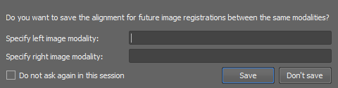
Figure 1812. Save Registration Results dialog window
Save Registration Results
If multiple cameras are used (two cameras each on a different camera port), one camera with two different objectives is used or one camera having a different zoom value (defined in two optical configurations) is used, Save Registration Results dialog window appears after clicking in the Registration Wizard dialog window. Enter the modality name and choose whether or not to save the alignment for future image registrations between the same modalities.
Opens a dialog window where you can manage registration results (e.g. used for aligning images by Image > Channel Alignment and Registration > Multimodal Image Registration). Camera port, objective, relay lens zoom, microscope zoom and microscope body name are stored.
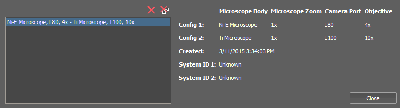
Figure 1813.
This command displays a window with the unmixing options. Unmixing of a spectral image can be performed if you click the Unmix button.
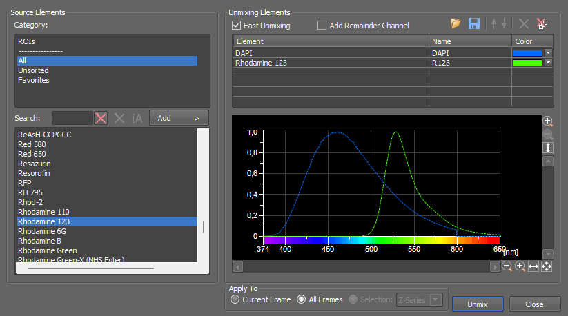
Figure 1814.
Resulting name and color can be adjusted by clicking inside the table. When all unmixing elements are added to the table, the list can be saved as an XML file using the nearby Save Unmixing Settings button. Load the saved table by the Load Unmixing Settings button.
Unmixing tasks can be demanding. If so, you can select the Fast Unmix check box to perform simplified unmixing, and you will get the result faster.
A channel that will contain the deviation data can be appended to the resulting image. Just check this box.
This command performs spectral unmixing of the current image using most recent Image > Spectral Unmixing Setting command settings.
This command opens the Blind Unmixing window:
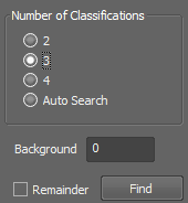
Figure 1815.
Define number of classifications for unmixing.
Define value of background in the image.
Performs Blind Unmixing and creates new multichannel image.
Opens a window which controls and manages the stored spectra.

Figure 1816.
Choose one of the groups in the Category area. All dyes present in the selected group are displayed in the Spectra area. Select a spectra or find it using the box. Then use the controls in the top right corner to manage the selected spectra. You can backup user spectra to an external *.xml file (Backup User Spectra), restore them again (Restore User Spectra), import previously stored spectra (Import Spectrum) export the existing ones into an external text file (Export Spectrum). User defined spectra can also be removed (Remove Spectra) or renamed (Rename Spectrum).