6D

Temperature/Gas
Volume Contrast
HDR
ImageJ Bridge
Bio Analysis
Single Particle Tracking
Filter Particle Analysis
N-STORM
N-SIM
Alveole Leonardo
EDF
Layer Thickness Measurement
Ratio, Ca2+, FRET
Metallography
Layer Thickness Measurement
Weld Measurement
Concrete


Saves the currently active image to the defined Input location in tif format
Starts the defined ImageJ Executable (*.exe) as a new process and passes the specified Parameters and the path to the Macro to it.
Waits for the process to end.
Saves the Output image and opens it in NIS-Elements.
Display the focused image.
Select the Edit Area in Focused Image command.* The cursor changes.
Draw an area inside the focused image which should be affected. Finish drawing by right-click.
Use the mouse wheel or arrow keys to browse Z slices within the area.
Finish the procedure by right-click or Enter.
Select a mono image from the pull-down menus for each FRET channel. Their previews appear.
Select a method, calibrate the module, modify the coefficients (similarly as if capturing the FRET image - see Applications > Ratio, Ca2+, FRET > Capture FRET Image). Confirm the settings with .
A new FRET image is created and opened within the application screen.
Insert the D-labelled sample. Press the Capture Donor Only Sample button.
A new image will be captured and named “Donor”.
Insert the A-labelled sample. Pres the Capture Acceptor Only Sample button.
A new image will be captured and named “Acceptor”.
Press the Calibrate button to display the calibration dialog. (Or run this command.) The FRET Calibration window appears.
Select the “Donor” image and the “Acceptor” image in the appropriate pull-down menus.
The Define ROI and the Define Background ROI buttons distinguish the foreground/background parts of the images.
Draw the background/foreground ROIs.
Confirm the calibration by .
Left mouse button marks the beginning and the end of a line section. This section will be erased.
Left mouse button + Ctrl marks the beginning and the end of a new air void.
Left mouse button marks the beginning and the end (left to right) of a line section of a detected air void. This section will be erased.
Left mouse button marks the beginning and the end (right to left) of a new air void.

(requires: 6D)
Captures multi-dimensional ND2 image data-sets.
See About ND Acquisition and Multi-channel Acquisition.
Note
Due to safety reasons, changing of objectives during a single ND experiment is not allowed.

(requires: 6D)
This command runs the Multipoint Set Acquisition window which runs one ND Experiment several times over a pattern of XY stage positions. All options except the ones described below matches the options of a simple multi-point acquisition. See Multi-point Acquisition.
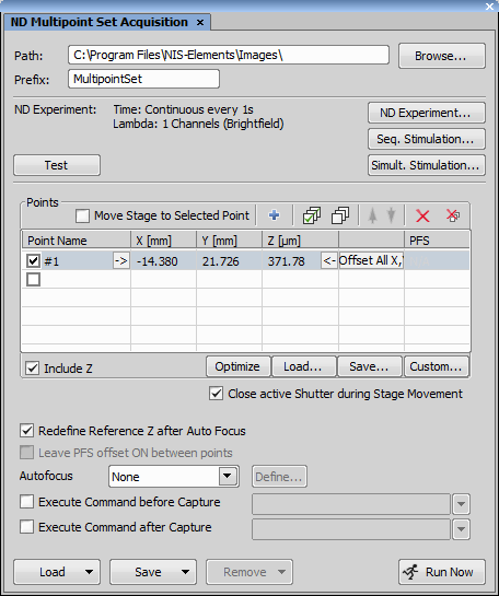
Figure 2057.
Enter a path for saving files made by ND acquisitions. Use the Browse button to search for a proper location.
Define a prefix common for all saved files.
Shows overview information about lower ND acquisition subset. Press the ND Experiment button to open an Multipoint Set Acquisition window which selects parameters of the lower ND acquisition subset.
(requires: 6D)
If more than one stimulation devices are connected to the system, this command enables you to select the default one which will be used during stimulation experiments.
(requires: 6D)
This command displays a window where it is possible to setup a sequential stimulation/bleaching experiment.
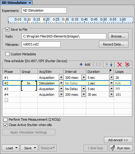
Figure 2058.
Columns
To specify the experiment, you have to define one or more phases (rows) and adjust values in the following columns:
Phase number. To add a new phase, click inside the check box.
You can group several phases of the experiment and set number of repetitions. Select two or more adjoining phases (holding Shift) and press the  button. Then, double-click the first row and specify the number of repetitions.
In this column, specify the phase type: Acquisition, Stimulation/Bleaching (these two are equal), Waiting.
Specify the interval between two actions of the phase.
Specify the overall length of the phase.
Specify the total number of actions of the phase.
Note
The Interval, Duration and Loops columns are dependent. If you specify two of them, the third will be calculated automatically.
Commands
Check this item to let the application automatically perform Time Measurement.
Check this item to close current active shutter in time between two captures.
See About ND Acquisition for description of the dialog options common to ND acquisitions.
See also Combined ND Acquisition.
(requires: 6D)
This command displays a window where it is possible to setup a simultaneous stimulation/bleaching experiment. Define the two simultaneous actions within the control window and press .
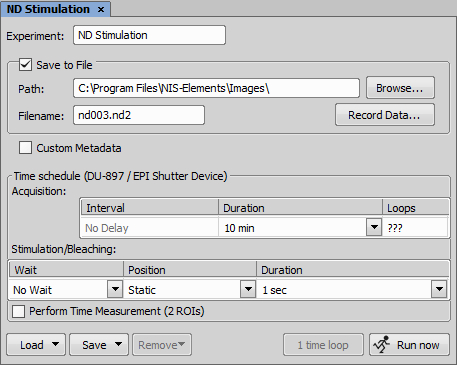
Figure 2059.
The interval parameter is always set to No delay. Set either Duration or Loops in order to specify the length of the captured time-lapse image.
The Wait value specifies time from the beginning of acquisition to the start of stimulation/bleaching. You can also select the Manual value to operate the stage manually during stimulation experiment. The manual option also defines the Position of stimulation ROI as static or manually repositionable. The Duration can be also set in manual mode.
Note
The Free Point Stimulation is supported only for a Stim. Point ROI. If any other stimulation ROI is used, then a warning message box is displayed when the Run now button is clicked.
See About ND Acquisition for description of the dialog options common to ND acquisitions.
See also Combined ND Acquisition.
(requires: 6D)
This command opens the ND Stimulation Parallel panel allowing parallel camera recording during stimulation with a stimulation device such as a DMD (Mightex, Mosaic), Galvo XY, or FRAP. The user can choose X number of phases on Y stimulation devices, either periodically repeating or continuous. It is a software triggered process which simply scans the given ROI (or in case of DMD it shines into it) either using or not using a time interval. Collisions in the stimulation phases (e.g. one device used in multiple phases in overlapping cases) should be avoided.
Name of the experiment.
If checked, another area is revealed enabling the user to type in or Browse the path where the files will be saved. Filename specifies the name of the file and its suffix can be selected from the drop-down menu.
Opens the Recorded Data dialog window enabling to choose which data are to be recorded and to optionally set Periodic Recording with a defined frequency.
If checked, another area is revealed enabling the user to edit custom metadata and use them in the experiment. Clicking on opens the Edit Custom Metadata dialog window (see Custom Metadata for details). The first drop-down menu selects the metadata set. Once it is selected, all the metadata contained in the set are loaded and can be used.
Selects the optical configuration used for acquisition.
The total duration of the experiment can be specified either by a time interval or by a number of frames.
Sets the time interval for the acquisition period. If no interval is needed, use No Delay.
Stimulation phase area. To add another stimulation phase, click  Add Phase. To delete a phase, click on in the top right corner of the phase.
Clicking on opens a dialog for selecting a previously created stimulation configuration.
Sets whether the stimulation is continuous or periodic.
Sets the stimulation phase start point.
Sets the stimulation phase duration.
If the stimulation phase is switched to Periodic, the stimulation period (pulsing) can be set here.
If the stimulation phase is switched to Periodic, the stimulation duration is set here.
Add Phase Adds another stimulation phase.
If checked, time measurement is performed and the Time Measurement dialog window opens.
Loads the experiment definition from a previously saved file.
Saves the experiment definition to a file.
 Run now
 Runs the parallel stimulation experiment.
(requires: Stage Incubator)
This function selects alternative (3rd party) interface for controlling incubation phases of ND experiments.
Opens the VC Capture dialog window used for creating a single volume contrast image after capturing a Z-Stack of a bright field. The number of the Z frames and the Z step size are determined automatically depending on the condition of the objective lens and camera.
Sets the optical configuration used for the capture.
Shows the Z-Stack size to be captured. For example “3 x 0.625 µm” means that three Z planes with a step size of 0.625 µm will be captured.
Specified the wavelength for the capture.
Defines the algorithm parameter influencing the background removal. The lower the number the more of the background is removed. Click on the  Recommended button to set the recommended value.
 Run
Run Executes the capture using the current settings.
Opens the VC Capture without Reconstruction dialog window which is used to capture a Z-Stack of a bright field. Volume contrast image is not created automatically but can be created later using Applications > Volume Contrast > Create VC Image from Current ND. This function is useful for adjusting the best parameters (“Well surface” and “Background level”) for samples as these parameters can be used for background shading correction.
Sets the optical configuration used for the capture.
Shows the Z-Stack size to be captured. For example “3 x 0.625 µm” means that three Z planes with a step size of 0.625 µm will be captured.
Specifies the wavelength for the capture.
Opens the ND VC Acquisition dialog window used to acquire an ND image with a combination of time, multipoint and large image after creating a volume contrast image from a Z-stack on each frame.
Captures a time dimension together with the Z-Stack. A new tab called Time Sequence is added to the left panel. Click on it to define the timelapse.
Captures a Z-Stack on each multipoint. A new tab called Predefined Points is added to the left panel. Click on it to define the multipoints.
Captures a large image Z-Stack. A new tab called Large Image is added to the left panel. Click on it to define the large image.
Reconstruct Now makes the volume contrast image immediately while Reconstruct Later creates an nd2 Z-Stack image which can be converted to the volume contrast image later using Applications > Volume Contrast > Create VC Image from Current ND.
Sets the optical configuration used for the capture.
Shows the Z-Stack size to be captured. For example “3 x 0.625 µm” means that three Z planes with a step size of 0.625 µm will be captured.
Specified the wavelength for the capture.
Defines the algorithm parameter influencing the background removal. The lower the number the more of the background is removed. Click on the Recommended button to set the recommended value.
Specifies the filename, and whether the image is saved or not. A folder where the image is saved can be specified after clicking .
Run Executes the capture using the current settings.
Opens the ND VC + Fluorescence Acquisition dialog window used to acquire an ND image with a combination of time, multipoint and multi-channel (volume contrast + fluorescence).
Captures a time dimension together with the Z-Stack. A new tab called Time Sequence is added to the left panel. Click on it to define the timelapse.
Captures a Z-Stack on each multipoint. A new tab called Predefined Points is added to the left panel. Click on it to define the multipoints.
Sets the optical configuration used for the capture.
Shows the Z-Stack size to be captured. For example “3 x 0.625 µm” means that three Z planes with a step size of 0.625 µm will be captured.
Specified the wavelength for the capture.
Defines the algorithm parameter influencing the background removal. The lower the number the more of the background is removed. Click on the Recommended button to set the recommended value.
This table is used for multi-channel acquisition. For more information please see Multi-channel Acquisition. The Focus Offset Setup enables parfocality adjustments for different filters (wavelengths).
Specifies the filename, and whether the image is saved or not. A folder where the image is saved can be specified after clicking .
Opens the Create VC Image dialog window used to convert the current ND image including Z-Stacks to a volume contrast image.
Note
The number of Z frames in the source ND image must be odd.
Shows the nd2 file calibration.
Shows the Z step.
Specified the wavelength for the capture.
Defines the algorithm parameter influencing the background removal. The lower the number the more of the background is removed. Click on the Recommended button to set the recommended value.
(requires: High Dynamic Range)
This command starts the Capture HDR Image function with all settings calculated automatically. The algorithm starts from the current exposure, finds high and low exposure times and the step count. As a result the application creates a standard (not multichannel/multiexposure) image.
(requires: High Dynamic Range)
Captures a high dynamic range image. Press to capture the HDR image according to the settings.
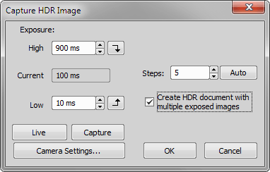
Figure 2060.
Set the highest and the lowest exposure values to be included in the capturing. The buttons next to the edit fields enables you to try the exposure times in live image (the buttons set the defined exposure time as current).
the maximum exposure time
indicates the current exposure time on live
the minimum exposure time
Define the number of steps for HDR capturing - how many frames the HDR image will be calculated from. Use the button to calculate optimal number of the steps for the current exposure range.
Select this option to create a multichannel image. Each channel will be named according to the exposure time used to capture it.
Starts live image.
Performs standard Capture command (not the HDR capture).
Displays the Camera Settings control window.
(requires: High Dynamic Range)
This command creates a HDR image from a ND2 file. The new HDR image opens in a separate window.
(requires: High Dynamic Range)
Selects source files for creating an HDR Image. The new HDR image opens in a separate window. If you check the Create Multiexposure Image option, a multichannel image is created.
(requires: High Dynamic Range)
Opens the Apply One Shot HDR dialog window used for enhancing the dynamic range on the currently opened image.
ImageJ Bridge is a master dialog which provides and shows all the image data to ImageJ software while ImageJ performs all the processing.
The Settings dialog window is used for defining ImageJ software path, parameters and the input and output folder. ImageJ application has to be installed first. See the example below where Fiji (image processing package distribution of ImageJ) was used.
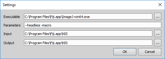
Figure 2061.
Path to the ImageJ executable file.
ImageJ parameters.
Input image path.
Path where the output image is saved.
Opens the Process Current Image dialog window used for image processing through ImageJ. After clicking the button, the following steps are performed:
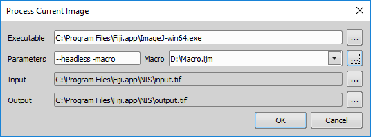
Figure 2062.
Path to the ImageJ executable file.
ImageJ parameters.
Path to a macro command file. This command can be assigned to a button in NIS-Elements.
Input image path.
Path where the output image is saved.
This command counts number of cells varying in time. See Cell Count Analysis.
(requires: Advanced 2D Tracking)
This command measures cell motility. Please see Cell Motility.
This analysis measures cell growth in time. Please see Cell Proliferation.
(requires: General Analysis)
Displays the General Analysis RGB dialog window. It allows to create a new binary layer defined as an intersection of the three RGB channels based on the RGB or HSI threshold values. All other features of the dialog window are the same as in General Analysis (see: Image > General Analysis).
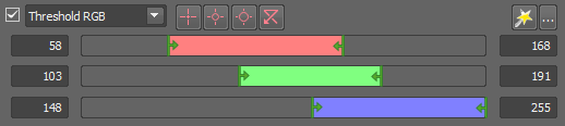
Figure 2063. RGB Threshold in General Analysis RGB
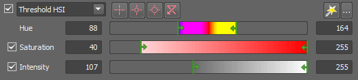
Figure 2064. HSI Threshold in General Analysis RGB
This command measures changes of cell distribution in time. See Wound Healing .
Imports a list of molecules from a *.roi file. See Applications--Single Particle Tracking--Import Molecule List.

(requires: Filter Particle Analysis)
This command runs the Filters module. See Filter Particle Analysis for detailed description of all features of the module.

(requires: N-STORM Analysis)
Opens the N-STORM dialog window for acquisition of STORM images. For more information please see N-STORM Acquisition and Analysis.

(requires: N-STORM Analysis)
Opens the Molecule Analysis dialog window used for localizing molecules.
For more information, please see Molecule Analysis.
(requires: N-STORM Analysis)
Opens the N-STORM Analysis Module within NIS-Elements. For more information about this module, please see N-STORM Acquisition and Analysis.
Creates a widefield image from a SIM image. Open a SIM image and run this command. Create Widefield from SIM dialog window opens. X and Y tiles are automatically detected from the image metadata. Click to create an averaged widefield image.
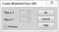
Figure 2065.
(requires: Local Option)
Opens the Alveole Leonardo dialog window.

(requires: EDF Module)
When the method is selected and the sequence is aligned, the only thing to do is to run the Applications > EDF > Create Focused Image command. The focused image will be created and appended to the ND2 file (when the ND2 file is saved to disk the focused image is included).
Dialog Window Options
Sets the method for the Z reconstruction. This reconstruction takes all Z slices and their focused image to create a 3D model of the whole scene called Z-Map. The Balanced method brings more consistent results with less noise and artifacts when compared to the former faster method (Original). If the Z-map calculation is not necessary for your task, select None to speed up the EDF image acquisition.
Places the lowest Z slice in the zero level, e.g. for better interpretation.
The original absolute Z coordinates remain intact.
Check this option if you do not want to see this dialog in the current session again.

(requires: EDF Module)
Creates a new document containing one EDF focused image (Z-stack from the source image is merged into a single frame).

(requires: EDF Module)
Measures within the Z-profile graph. Please see the description of the View > Analysis Controls > EDF Z-Profile .

(requires: EDF Module)
This command displays the anaglyph view of the current data-set. The focused image must have been created before. See Extended Depth of Focus.

(requires: EDF Module)
This command displays the surface view of the current data-set. The focused image must have been created before. See Extended Depth of Focus.
(requires: EDF Module)
This command opens a sequence of images and creates an ND2 file out of it.
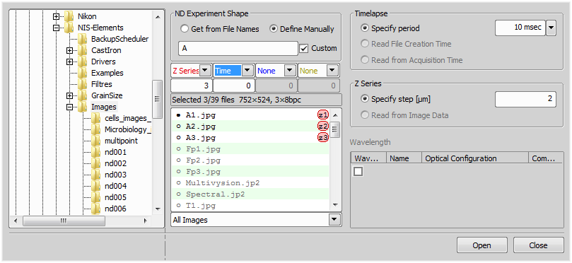
Figure 2066.
Specify the folder which contains sequence images.
Mark this button to define ND2 file from file names.
Mark this button if you want to define the files manually.
If you want to edit the name pattern manually, check this item and the text field on the left side of this option becomes editable. Edit the text or enter a new name pattern.
Set the dimensions of ND2 file (Time, Z Series, Wavelength, Multipoint). Specify number of dimension frames in file sequence in the field below.
This portion of the window displays a list of all available files. Select the file which will represent a first frame in ND2 file by double-clicking its name or click on the point before the file name.
Set Timelapse period value. Specify the exact value from the pull down menu or select to use File Creation Time or Acquisition Time.
Set Z Series step as value (µm) or select to use the Z Series step from Image Data.
Define name of the channel. Define name of the existing optical configuration or start defining a new one. Choose one of the seven predefined colors or brightfield option as a color of the channel. You can also select the More option to define a custom channel color.
Opens the selected sequence of image as a ND2 file according to the given properties.
(requires: EDF Module)
This command aligns the current Z series in order for the EDF to work properly.
(requires: EDF Module)
This advanced option enables you to draw an area inside the image and select the Z slice to be used in the resulting focused image.
* - when you have the area defined, the selection can be inverted by pressing G.
(requires: EDF Module)
This function enables the user to handle the background of a Z-series surface image viewed in the EDF Surface View (Applications > EDF > Show Surface View ). After the focused image is created, you can invoke this command. The following dialog appears:
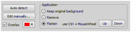
Figure 2067.
First, you have to detect the background. Click to perform the autodetection. If the results are not fully satisfying, or in any other case, choose to open the ROI editor. Detect the background using the tools available and then press the Tab key or click  Exit Editor to close the editor.
See Binary Editor.
Check Overlay and set the color of the overlay for better visualization of the edited layer.
Finally choose how to process the background in the Application section. Remove option deletes the detected background area. Flatten will set all the background Z-coordinates to zero so that the background will form the zero level which can be moved in the Z dimension or . If you do not want any of the mentioned options, select Keep original background.
(requires: EDF Module)
This command displays the Z map of an ND document which contains the Z dimension.

(requires: EDF Module)
The Real Time EDF command is integrating the whole functionality of EDF. It captures a Z-sequence, aligns the images (optionally), and creates the focused image. When the command is invoked, the RealTime EDF dialog appears. Check, whether to align the images or not. See also Real Time EDF.
(requires: EDF Module)
The Real Time EDF Manually command is integrating the whole functionality of EDF. It makes the focused image from a Z-sequence captured from the Live stream during manual Z movement. When the command is invoked, the following dialog appears. Check, whether to align the images or create a Z-Map and click .
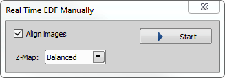
Figure 2068.
(requires: Local Option)
Opens the Layer Thickness Measurement dialog window. See Layer Thickness Measurement.
(requires: CA FRET)
This command turns on ratio view of the current image. Ratio view displays the image as a ratio of its two channels. A color scale appears in the left corner of the image.
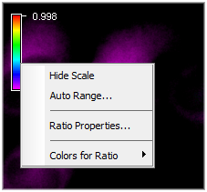
Figure 2069.
Context Menu Commands
Hides scale.
Sets autorange to the ratio scale.
Opens the Ratio Properties dialog.
Opens a submenu with color schemes. You can select which color scheme will be use for rendering of ratio component.
See Also
Applications > Ratio, Ca2+, FRET > Ratio Properties
(requires: CA FRET)
This command invokes the following window where properties of Ratio View can be set.
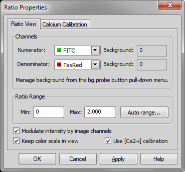
Figure 2070.
These two combo boxes determines the source channels which the ratio will be counted from. Names of all available channels of the current image can be selected.
The offset value is subtracted from the corresponding channel before the ratio will be counted.
The range displayed on a ratio color scale is defined by the Minimum and Maximum values. Write the values inside the edit boxes or use the Auto Range button to fill them automatically. The system will count a reasonable range according to the image scene.
By default it is switched on and shows the ratio modulated by the average intensity of the selected channels. The user can switch the modulation off and display the raw ratio of two selected channels.
This check box keeps the color scale in view when the image is zoomed in.
This check box enables the user to use the Ca2+ calibration.
Note
This dialog window allows navigating between other image frames and check ratio in any pixel of any frame without closing the dialog.
(requires: CA FRET)
This command turns on the Calcium view. For more information about Calcium see FRET.
(requires: CA FRET)
This command opens the Ratio Properties window.
For more information see [Ca 2+] Ion Concentration Measurement.
(requires: CA FRET)
This function toggles the Ph visibility. To show the Ph view, check the appropriate item in the Ratio etc. pull down menu. Uncheck the item to hide it.
Ph is only a default name, but you can define any other name of measured value using Applications > Ratio, Ca2+, FRET > Titration Calibration in Vitro. If the Ph View is turned on, a new channel with Ph values is added into image. A scale bar which shows minimal, maximal and mean values of measured value and color gradient is inserted into the top left corner of the image window.
(requires: CA FRET)
This command opens the Titration Calibration in Vitro window, which defines the calibration curve:
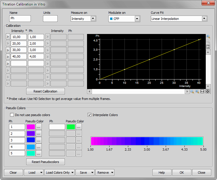
Figure 2071.
Define and enter a name for measured value. Default name is .
Defines units of measured values.
Defines on which value the calibration is performed:
Intensity of selected channel.
Ratio value according to ratio View Properties.
Define a channel with measured values.
Define the method for curve fitting.
Set intensity values. Use the red probe displayed in the image, adjust its size and position and click next to your edit box to fill it with the intensity value obtained from the probe.
Enter a measured value for each point of the calibration curve.
Deletes all calibration values.
Shows the calibration curve. You can zoom in/out horizontally or vertically using the buttons in the top right and bottom right corners.
If turned on, pseudo colors are not used and a grayscale gradient is used instead.
Check this item to change the sequential color scale to gradient color scale.
Measured value for one point of the color gradient.
Shows the selected color and enables the user to redefine it for the measured value.
Resets all pseudo color definitions and sets the default color gradient.
Clears all definitions in the dialog.
Loads the saved configurations including colors from an .XML file or reuses them from an image file (Reuse from Image File). If the definition is saved as New... in the drop down menu, it will be listed here.
Loads just the color definition from an .XML file or from an image file.
Saves configurations into an .XML file, into the drop-down list () or overwrites an existing configuration from the list. Configurations saved to the drop-down list are stored per user.
Displays a list with the names of saved configurations. Selected configuration will be removed.
(requires: CA FRET)
This command processes image documents using a custom equation.
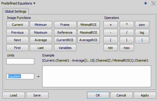
Figure 2072.
You can insert some basic equations from the Predefined Equations menu (see Custom Equation for examples). Channel names can contain special characters (/,-,;) and blank spaces. Maximum number of the custom equations is 20. Equation can be stored and reused from a text file or from an image file. Number of the equation channels is 12. Global variables can be used in the equations.
It is also possible to use LUTs for the equation channels.
Once the equation view is created in the image, you can blend the equation image with one or more existing channels. Right-click the equation channel tab and select Equation View Settings.... Select the Blending Options tab, mark channels you want to blend and define the share (percentage) in the resulting view. The context menu over the channel equation tab also enables the user to Convert Equation to Mono Channel / Floating Point Channel and to Extract as RGB Snapshot / Floating Point Image.
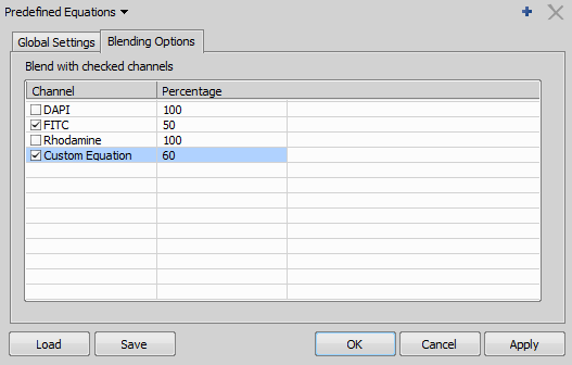
Figure 2073.
Press the buttons to insert the available functions to the custom equation. A dialog window appears where you shall define parameters for the selected function. E.g.:
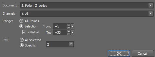
Figure 2074. Example of selection of possible parameters
Choose which channel is processed.
Define range of processed frames of an ND document: All Frames, or Selection (From, To) can be selected. If you check the Relative option, the range can be defined relatively.
Define which ROIs are processed.
Define index of a frame to be processed by the function. If you check the Relative option, the index can be defined relatively.
Press the button of a corresponding operator to insert it to the custom equation.
Define in which units is the equation calculated.
Write the custom equation into this field. Use the functions and operators provided in the window. You can also edit the equation manually.
Loads previously saved settings from an external file.
Saves current settings to an external file.
(requires: CA FRET)
This command defines custom equation for processing the live image. The Custom Equation window appears.
See Applications > Ratio, Ca2+, FRET > Add New Equation View for more information about the tools in this window. Only some of the tools are disabled due to processing of the live signal.
(requires: CA FRET)
This function removes defined equation view from live.
(requires: CA FRET)
Any image can be converted to a FRET image. Either run this command or right click the image and select FRET View. Then run the FRET Method command from the context menu of the image. The following window appears. Assign the channels to the emission type (Da, Dd, Aa, Ad), and select the FRET method. Calibrate the module or enter the FRET coefficients by hand.
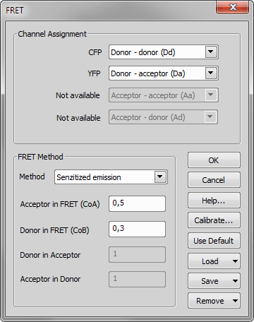
Figure 2075.
See Also
FRET
(requires: CA FRET)
Run the Applications > Ratio, Ca2+, FRET > Capture FRET Image command to display the main FRET control window. Select the appropriate settings and capture the FRET image by the Capture FRET button.
The FRET control window consists of several sections. In this section, optical configurations which will be used during the acquisition should be assigned to FRET channels.
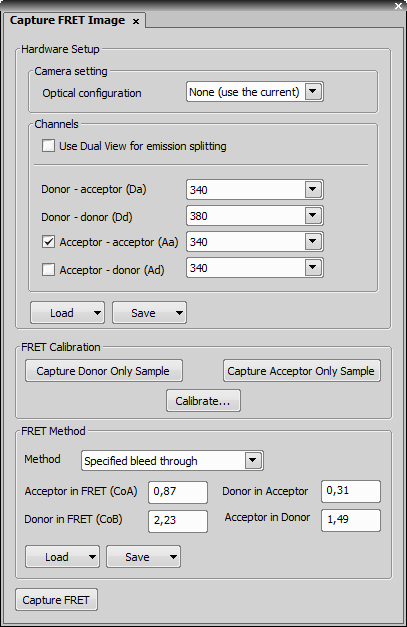
Figure 2076.
In this pull-down menu, select an optical configuration that contains Camera settings which shall be used during the FRET image acquisition. If None is selected, the current camera settings will be used.
The FRET image can contain 2-4 channels. Here you can assign an optical configuration to each of them. It is recommended that the optical configuration contains only the filter changer settings.
If the Dual View device is available, it can be used for channel splitting. Then, only one optical configuration for each excitation wavelength will be used.
Note
The Dual View device splits the emitted light to two beams filtering different wavelengths, and each of them is captured by only a half of the camera chip.
The channels settings may be saved to the system by the Save button. Once saved under some user defined name, this name appears in the Load pull-down menu ready to be loaded. The settings can also be loaded from an external FRET image.
The calibration work-flow is described in Applications > Ratio, Ca2+, FRET > FRET Calibration command description.
In this section, select one of the four available FRET methods.
There can be 2 or 4 coefficients used according to the selected method. Their values are results of the calibration. If the calibration was not performed, you can put the coefficients in by hand. The coefficients settings can be saved/loaded similarly to the channels settings.
(requires: CA FRET)
This command defines the donor channel in Timelapse ND2 files.
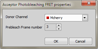
Figure 2077.
All channels present in current image are listed in the combo box. Select which channel is donor.
Use the arrow buttons to define the exact number of frames which were captured before bleaching.
Percentage intensity (I) of the new channel is obtained using the following formula where I0 is the initial frame intensity and In is the current frame intensity.
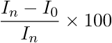
Figure 2078.
(requires: CA FRET)
The FRET image can be created from images saved on hard disk too. Run the Applications > Ratio, Ca2+, FRET > Create FRET Image from Files command. A window appears. The FRET image creation principles are the same as if capturing the FRET image except that you provide the module with mono images from hard disk (instead of capturing them via a camera).
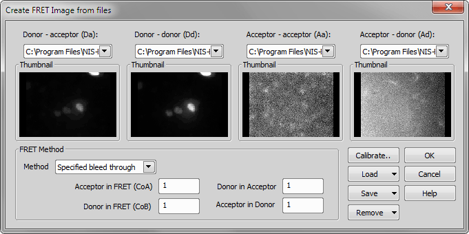
Figure 2079.
See FRET.
(requires: CA FRET)
Separate images of the D-labelled and the A-labelled samples must be acquired in order to calibrate the FRET method correctly. Run the Applications > Ratio, Ca2+, FRET > Capture FRET Image command to display the FRET control window.
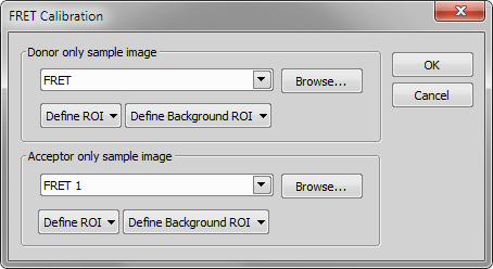
Figure 2080.
Note
Any image file can be used for the calibration. The pull down menu displays the currently opened images. Other images can be reached via the Browse button. If a non-FRET image is used, a window appears where you should map the image channels to FRET channels and select the FRET method.
(requires: CA FRET)
This command displays the current FRET coefficients and enables the user to adjust them manually.
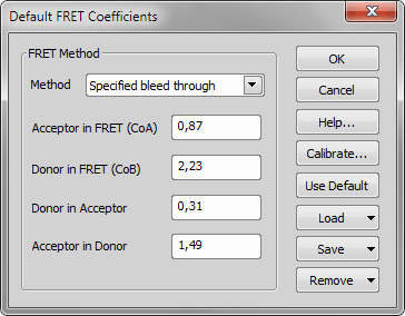
Figure 2081.
See FRET.
(requires: Metalo - Cast Iron Analysis)
This command starts the Metallography - Cast Iron application layout. Please see Metalo - Cast Iron Analysis for further details.
(requires: Metalo - Grain Size Analysis)
This command starts the Metallography - Grain Size application layout. Please see Metalo - Grain Size Analysis for further details.
(requires: Layer Thickness)(requires: Local Option)
Opens the Layer Thickness Measurement dialog window. See Layer Thickness Measurement.

(requires: Local Option)
Opens the Measurement Explorer panel.
See also Measurement Explorer.

(requires: Local Option)
Opens the Measurement Sequencer - Definition panel used for the preparation of advanced sequential measurement definitions.

(requires: Local Option)
Opens the Measurement Sequencer - Run panel used for executing the measurement definitions previously defined in the Measurement Sequencer - Run window.
(requires: Local Option)(requires: Concrete)
This command executes the concrete measurement. At first a wizard appears where the Measurement name has to be filled. A new directory with this name will be created in the shown Report directory. The measurement report will be saved to this directory. It is required to insert a unique measurement name in the scope of the Root directory otherwise the wizard will not proceed.
Note
Please, do not use “test” as the measurement name. It is reserved for testing purposes. The reports in the “test” directory will be overwritten without notice.
After the measurement name is inserted, prefocusing on the concrete sample must take place. You will be prompt to focus manually (if the three-point prefocus is selected, you will need to focus three-times, see Focusing in the Measurement tab in Applications > Concrete > Options). The focusing can be done by the mouse wheel or by the joystick wheel. Click and confirm the calibration of the document by clicking . Then the Measurement progress window appears. Information about the measurement progress is displayed on the left. The top bar shows the task progress in the scope of the current concrete sample and the bottom bar in the scope of the whole measurement.
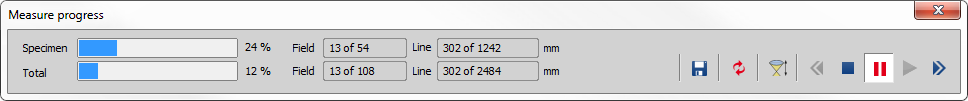
Figure 2082.
 Save current image...
 Saves the current image to a .jpg file.
 Refresh detection
 Refreshes the current detection.
 Focus manually...
 Manually focuses on the current measurement step.
 Previous step
 Moves to the previous step in the measurement sequence. It is enabled only if the  Pause button is pushed.
 Stop
Stop Finalizes the measurement and creates a report.
Pause Pauses the automatic measurement.
Play Starts the automatic measurement.
 Next step
 Moves to the next measurement step. It is enabled only if the Pause button is pushed.
Keyboard shortcuts used while measuring:
Secondary mouse button.
Ctrl + secondary mouse button.
Middle mouse button.
Ctrl + middle mouse button.
Primary mouse button.
Primary mouse button (left to right).
Ctrl + primary mouse button.
Primary mouse button.
(requires: Local Option)(requires: Concrete)
Opens the concrete Classifier definition. The classification of air voids is based on a neural network which must be “taught” first in order to produce reliable results. During the classifier definition, every color shade in the image (either representing background or air voids) should be clicked at least once (i.e: if you have a two-color background, click on each color at least once). The classifier is applied only if both the air voids (foreground) and the background were defined.
Once the classifier is taught, click . The current image will be classified and a binary layer with the objects detected as air voids will be displayed over it. You can toggle the binary layer visibility using .
Warning
When testing the classifier by the button, inaccurate results may appear. This happens when the learning mechanism of the neural network gets confused. In such cases, determining additional air voids/background points should help. Or reset the classifier completely and teach it from scratch. Once the test passes successfully, the classifier can not fail during the measurement.
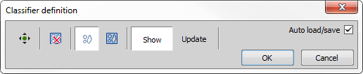
Figure 2083.
 Live
Live Turns on the live signal from the camera and activates the joystick. You can move the stage and look for an optimal texture suitable for the classifier definition.
 Reset classifier
 Resets the current classifier.
 Define air voids
 Use this button to teach the classifier to recognize air voids - click in the image on the air voids several times.
 Define background
 Use this button to determine the background - click in the image on the background several times.
Toggle the binary layer visibility.
Updates the classifier with the new definition.
If checked, the classifier settings will be remembered for future use and it will be loaded automatically when NIS-Elements is started the next time.
Confirms the settings and closes the Classifier definition window.
Discards all the settings and closes the Classifier definition window.
(requires: Local Option)(requires: Concrete)
This command opens the concrete Settings dialog window containing the following tabs.
Specimen
In this tab, set the number of concrete samples (specimens) to be measured, their dimensions, the length of the traverse lines and their layout over the specimen. When you press the button, values which are needed to fulfill this Euronorm requirements will be set.
Specifies the number of samples to be measured.
Specifies the length of the specimen.
Specifies the width of the specimen.
Specifies the top and bottom non-metering margins of the specimen.
Specifies the left and right non-metering margins of the specimen.
Specifies the percentage of the volume paste present in the specimen.
Specifies the total length of the traverse line.
Specifies the spacing between the traverse lines.
Specifies the number of lines on margins.
Sets all the specimen parameters according to the Euronorm EN 480-11.
Measurement
Editing method of the detected air voids, XY stage settings, automatic focusing method, and the result filtering parameters can be adjusted in this tab.
Classic
CAD system
Check Manual XY if you use a manual XY stage.
To measure only along the X axis, check Measurement along X.
Check User-defined XY scanning start position to set a new scanning starting position based on the current stage coordinates. Click to set the new scanning start position. To move the stage to this position, click .
When scanning a concrete sample, the system focuses repeatedly every n-th frame (n=step). If the concrete sample is well prepared (perfectly flat with constant thickness), you can set the step to 5 or higher. If it is rather oblique, check Use three-point prefocus.
Cleaning factor specifies the minimal size of the detected air voids in micrometers. Air voids smaller than that will be omitted. On the contrary, if an empty space between two air voids is smaller than the Filling factor value, the two air voids will be merged into one.
Note
The Cleaning factor is applied first.
Report
At the end of each measurement task, a report is created containing the measurement results. The report consists of several files, all placed into the Root directory. Here you can specify the destination file names.
Directory where the report files will be placed.
Path to a predefined .rtf template.
Path to a predefined .xls template.
Specifies the name of the .rtf file.
Specifies the name of the .xls file.
Specifies the name of the .txt file.
Specifies the name of the histogram .bmp image.
Stores an image file containing the album of detected air voids. Each measurement frame is cropped so only a thin stripe containing the traverse line remains. These stripes are stitched together, labeled and saved to the album file. Measurement results can be verified visually using this image.
Specifies the name of the album .bmp image.
Lines
Graphic properties of the annotation objects used during the measurement can be set here.
Color and width of the traverse line can be adjusted here.
Color and width of the chord can be adjusted here.
Color and width of the help lines can be adjusted here.
Color of the air voids and paste can be changed here.
Voids smaller than the specified size can be highlighted with a selected color, width and length.
Other
If the motorized Z drive is not present in the system, an error message appears whenever the stage is being initialized. Here you can suppress this message.