
(requires: General Analysis)
With General Analysis, it is possible to make multiple binary masks on a single channel as well as to combine multiple masks by means of generic expression with powerful operators. It is also possible to calculate custom features. High interactivity enables viewing your result at any time. Check boxes enable viewing just the desired operations or analysis steps. Complicated sequences can be created in few minutes - e.g. color image processing, segmentation, binary image processing, object filtration and measurement, etc. Binary masks can also be mixed using a general expression. Any binary mask can act as a ROI (Region Of Interest) inside which measurement can be done (organelles, markers in cells, etc.).
General Analysis exists in two forms - as a part of the Jobs module local option (results go to the Jobs database and are automatically saved as Job Run) and as a local option of NIS-Elements available from the Image menu (results are shown in the Automated Measurement Results tab and are automatically deleted after closing unless they are saved). Except small details, the graphical user interface is almost the same in both forms.
See also: HCA Analysis.
Note
Any changes made to the color image are temporary. All operations (thresholding, processing, measurements, calculations, etc.) are made on the original (unaffected) image data. The General Analysis dialog setting is saved as a Recipe (see:  HCA/JOBS > Presets > Manage Recipes). Analysis results (for General Analysis from the Image menu) must be saved otherwise they are deleted after closing the results window. Results from General Analysis performed by Jobs are automatically saved in single Job Run.
Top Toolbar Options
The top buttons for General Analysis found in the Image menu are described in the Image > General Analysis section whereas General Analysis for Jobs is described in the Analysis chapter.
Analysis Palette
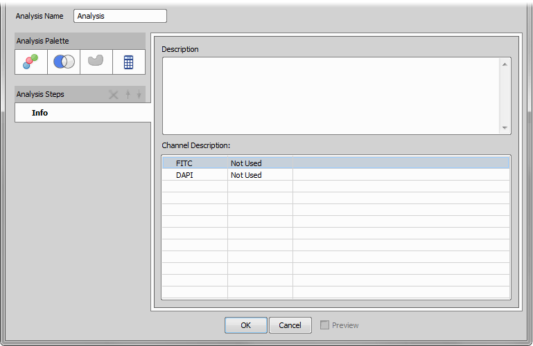
Figure 530. Info tab
This tab enables editing the General Analysis Description, viewing Channel Description and adding notes to each channel (3rd column in the bottom table). applies the current General Analysis setting and quits the window. Cancel closes the General Analysis window without using the current settings. Preview displays changes done in General Analysis inside the Preview window. These three last features can be found at the bottom of each general analysis tab.
 Add Channel tab
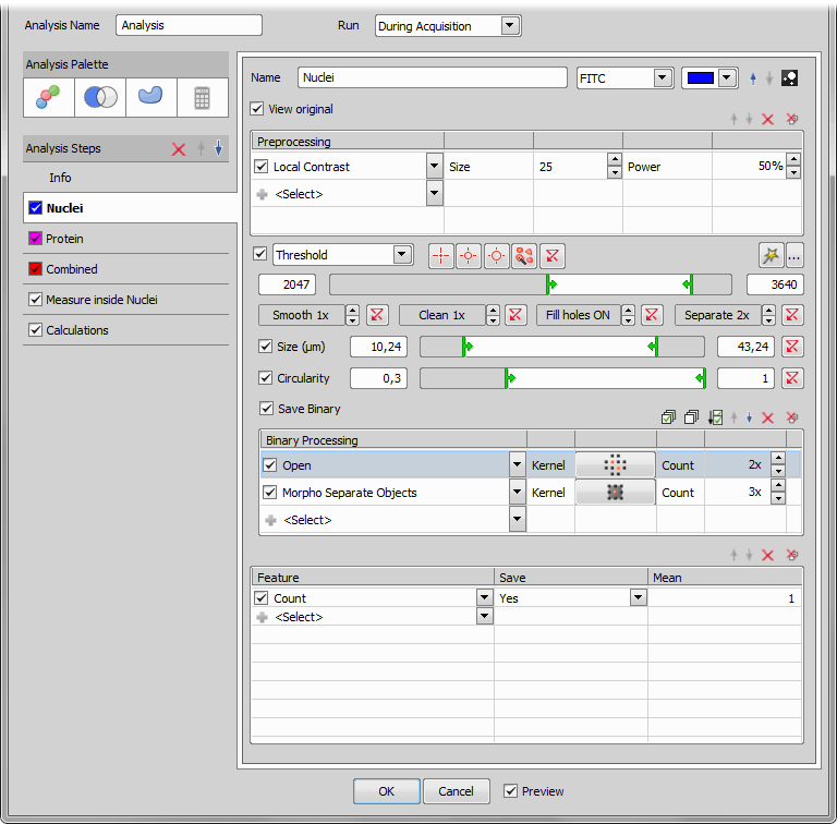
Figure 531. Add Channel tab
Add and name your new channel tab defined on a specified color channel. These two features can later be changed at the top of each channel tab, where you can also set the channel's color label. The  View Binary icon opens the Binary Layers panel showing all binary layers available.
 Move Layer Up/Move Layer Down icons moves the currently selected channel one step up / down in the Binary Layers panel. After defining parameters it may produce a binary mask as a result of channel segmentation and processing. When the analysis is executed it produces measurement on the mask (if made) and selected channel.
If the  Wizard button is clicked, the current Channel is marked with a wizard symbol and Thresholding parameters will be shown in the wizard area after the job is executed. Custom description to the threshold linked with its channel can be entered after clicking the button.
Note
The number of channels is limited to 40. However this number may not always be achieved. It depends on the maximal allowed value of the User Objects in the system process. This value is set to 10000 by default and can be changed in the registry key:
[HKEY_LOCAL_MACHINE\SOFTWARE\Microsoft\Windows NT\CurrentVersion\Windows\USERProcessHandleQuota]
 Add Combined tab
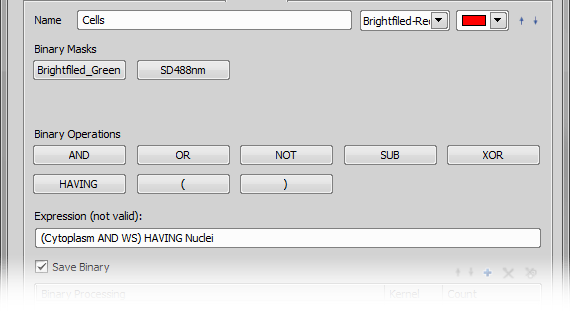
Figure 532. Add Combined tab
Combined tab is used to make binary images as a combination of existing (tabs above the current one) binaries (e.g. union, intersection of previously created masks). You can use the Binary Operations buttons to make an Expression which defines how existing binary masks are combined. The first row of buttons contains operands – the binary masks (from the tabs to left of the current tab). Below are the operators: AND – Intersection, OR – Union, NOT – Complement, SUB – Subtraction, XOR – Exclusive OR, HAVING and parentheses. AND, OR, SUB, XOR and HAVING are all binary operators: the are placed between operands. NOT is an unary operator placed before one operand. Parentheses should be used to dictate the order of operations. After defining the expression you can choose Binary Processing and Features to be calculated.
 Add ROI tab
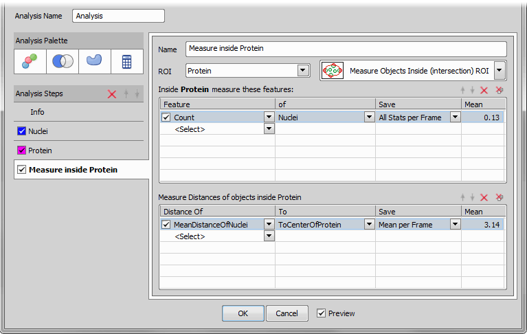
Figure 533. Add ROI tab
This tab measures features inside a selected binary. Choose the binary from the ROI combo box and select one of the methods handling objects touching ROI borders. Then add desired measured features below. You can also measure distances of objects to different objects and save these data together with the analysis results.
 Add Calculations tab
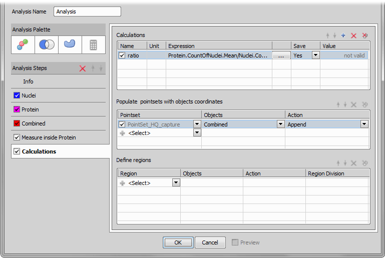
Figure 534. Calculations tab
Calculations
Adds a new tab called Calculations. These functions enable mathematical operations on measured data. By adding a new calculation and clicking the ... button you enter the Expression Definition window where you can write your expression using supported functions and operators:
| Function | Description |
|---|---|
| abs() | absolute value |
| acos() | arc cosine |
| acosh() | arc hyperbolic cosine |
| asin() | arc sin |
| asinh() | arc hyperbolic sin |
| atan() | arc tangent |
| atanh() | arc hyperbolic tangent |
| avg() | average |
| cos() | cosine |
| cosh() | hyperbolic cosine |
| exp() | exponential power |
| if(;;) | condition if |
| ln() | natural log |
| log() | logarithm |
| log10() | common logarithm |
| log2() | binary logarithm |
| max() | maximum |
| min() | minimum |
| rint() | round to integral value |
| sign() | sign |
| sqrt() | square root |
| sum() | sum |
| tan() | tangent |
| tanh() | hyperbolic tangent |
| Operator | Description |
|---|---|
| + | addition |
| - | subtraction |
| * | multiplication |
| / | division |
| ^ | square |
| < | less than |
| <= | less than or equal to |
| > | greater than |
| >= | greater than or equal to |
| == | equal to |
| && | logical AND |
| || | logical OR |
| != | not equal to |
For more information about writing expressions, please see Using Expressions.
Populate pointsets with objects coordinates
Populate pointsets with objects coordinates finds centers of objects in a selected binary and fills your point set with their coordinates. To use this function, your job definition has to contain the Stage XY Points > ![]() New Point Set task. Be sure you set the Action correctly. Append should be used in cases where the point set is firstly filled with all points and then more operations are preformed on this point set. Replace is used when a point position is found and the operation is performed immediately on it. Then it is overwritten by the next xy position where measurement is performed. For better understanding this function please see our two use cases: General Analysis in JOBS Module - Appended Point Set Use Case, General Analysis in JOBS Module - Replaced Point Set Use Case.
New Point Set task. Be sure you set the Action correctly. Append should be used in cases where the point set is firstly filled with all points and then more operations are preformed on this point set. Replace is used when a point position is found and the operation is performed immediately on it. Then it is overwritten by the next xy position where measurement is performed. For better understanding this function please see our two use cases: General Analysis in JOBS Module - Appended Point Set Use Case, General Analysis in JOBS Module - Replaced Point Set Use Case.
Define regions
This function automatically generates regions if your job definition contains the Large Images >  Region List task. Choose your Region list, specify on which layer the regions will be detected, choose between Append / Replace (described above) and select the Region Division (Per Frame / Per Object).
Analysis steps
 Remove Selected Tab
 Deletes the currently selected tab.
Move Up / Down Using these arrows you can move your tabs vertically in their inventory.
Main area options
Here you can choose one of the Preprocessing methods: Remove Average Background, Remove Dark Background, Remove Light Background, Subtract Background Using Contrast, Autocontrast, Local Contrast, General Convolution, Detect DIC Objects, Detect Edges, Detect Peaks, Detect Regional Maxima, Detect Regional Minima, Detect Valleys, Gabor Edge Detection, Gradient Morpho, Linear Close, Linear Dilate, Linear Erode, Linear Open, Close, Open, Low Pass Filter, Advanced Denoising, Fast Denoising, Median and Smooth.
 Kernel
 By clicking the kernel icon you can switch between different kernels. Each kernel icon represents a pixel neighborhood method, that is assigned to the preprocessing method selected. Every pixel of the image is then evaluated according to the selected kernel which influences the resulting image processed by the selected preprocessing method. Try to use different kernels to find out which one brings the best image results for your current capture setup.
Adjusts the intensity of the preprocessing method selected.
The threshold bar enables selecting low and high intensity thresholds. Only the pixels within this interval will be taken to make objects visualized as a binary mask. Threshold is optional in General Analysis. If it is skipped, only intensity features on the whole field of view are available. If the threshold is performed, it may be chosen not to save the binary image which is useful for temporary binary masks.
More information about thresholding can be found here: Thresholding.
Spot Detection uses mainly circular objects with same intensity values as a threshold.
For more information about setting up the Spot Detection parameters, please see: Spot Detection.
For information about this detection, please see Binary > Segmentation > Segment Tight Borders.
These tools function as filters. Use them to improve your image quality before processing. Use Smooth (to smooth rough edges) / Clean (removes small objects) / Fill Holes / Separate to get the objects.
 Reset
Reset This button resets the settings.
Position the sliders to restrict the area of the sizes of detected objects.
Position the sliders to restrict objects in your image with desired circularity.
Check if you want to save your binary layer together with your captured images.
Binary processing further alters the binary masks. The choice of operations is same as in NIS-Elements. You can choose some binary processing methods, set their kernel and intensity (Count).
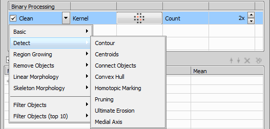
Figure 535.
When the Binary mask is fine-tuned it is time to set the features to be measured and saved into the database.
See Measurement Features.
Insert analysis info
You start with an empty dialog with the Info tab selected. Here you can insert description of the analysis.
Add relevant color channels to the analysis
Decide on which image channels the segmentation will be performed. Add these channels to the Analysis steps tab by the
Add Channel button.Define analysis of each channel
Adjust the preprocessing, segmentation, binary processing parameters and measurement features for the added channels. The resulting binary layers are displayed in the current image window. You can turn each layer on/off by the check box in front of the channel name.
If preprocessing has been applied, you can always display the original image by selecting the View original check box.
Note
Any changes made to the color image are temporary (only for Thresholding and Spot Detection) and all measurements are made on the original (unaffected) image data as well as saving.
Combine binary layers (optional)
You can perform logical operations processing and measurements on multiple binary layers. To do so, create a “combined” channel by clicking the
Add Combined Layer button and specify the parameters.Define ROI
Binary mask of one channel can be used as a ROI to restrict measurement on another channel. If this is the case, click the Add ROI button. In th ROI channel, again, specify the measurement features.
Define calculations
Click the
Add Calculations button to add the calculation step in the analysis. In this step you can define any mathematical expression using the features measured in previous steps of the analysis.Run the analysis
Click the button to apply the analysis to the current image. A new record will be appended to the list of performed analyses in the Analysis Explorer. The measured results are then accessible in the
View > Analysis Controls > Automated Measurement Results  window.
The possibilities of the General Analysis are best shown on a real example. In this case we are trying to find out how much of a protein gephyrin (in red) is present in positively labeled globular bushy cells (in green) using General analysis in NIS-Elements.
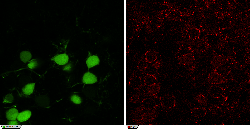
Figure 536.
The green channel “Alexa 488” shows globular bushy cells (GBC) in an anteroventral cochlear nucleus (AVCN) part of a rat brain stem. The red channel “Cy3” shows the protein gephyrin.
We start by opening the General Analysis dialog window ( Image > General Analysis) and adding the Alexa 488 as a new layer. This can be done clicking the Add Channel icon. We enhance the image using Local Contrast and then we define the threshold values to restrict our cells from the background and other objects. Just for better visualisation we also added Count as a Feature to know, how many objects are detected using the current settings.
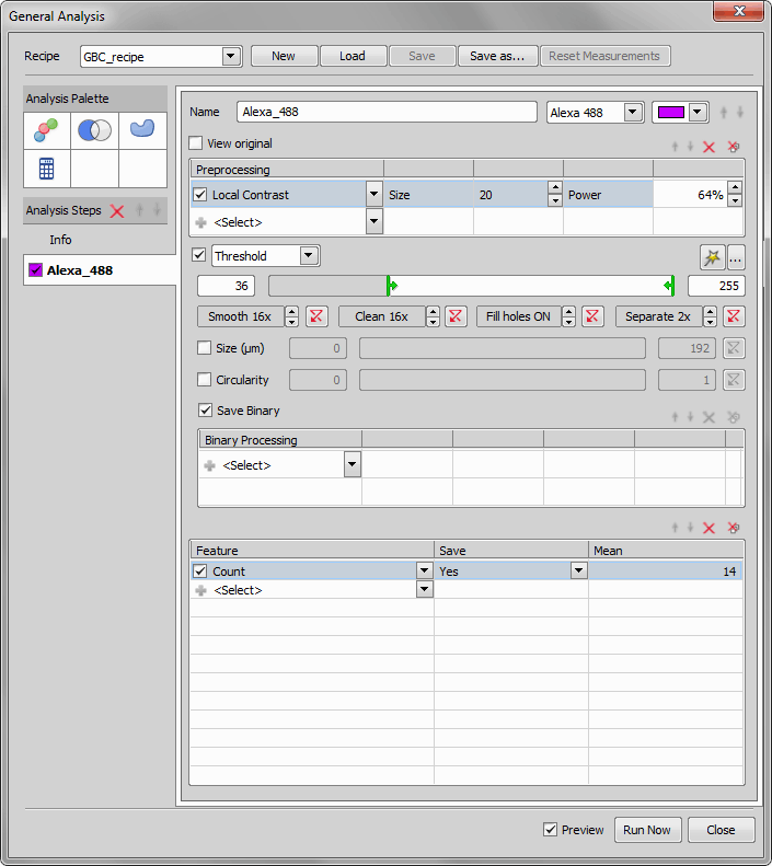
Figure 537. Parameters of the first channel.
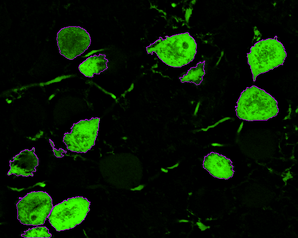
Figure 538. Resulting preview.
Now we can add the second channel and do thresholding as we did with the first one.
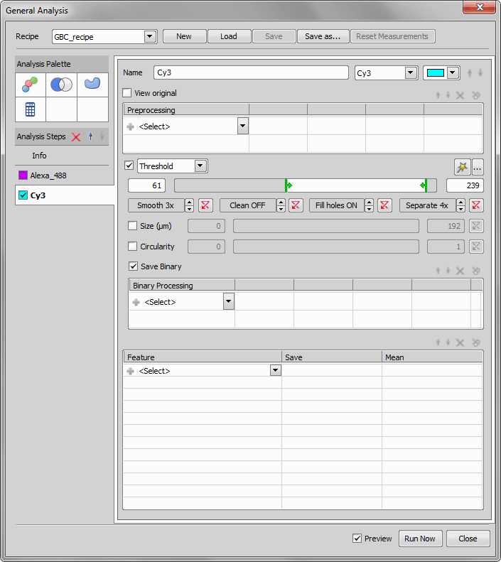
Figure 539. Thresholding the second channel.
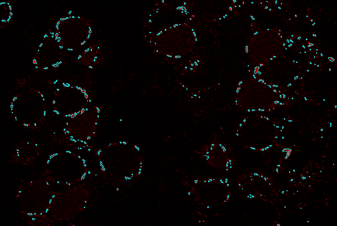
Figure 540. Resulting preview.
To find out which cells contain proteins we will combine both channels clicking the Add Combined layer icon and defining the expression as follows: Alexa_488 HAVING Cy3. This way we can create ROIs only with cells containing proteins.
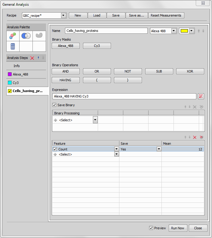
Figure 541. Combined tab settings.
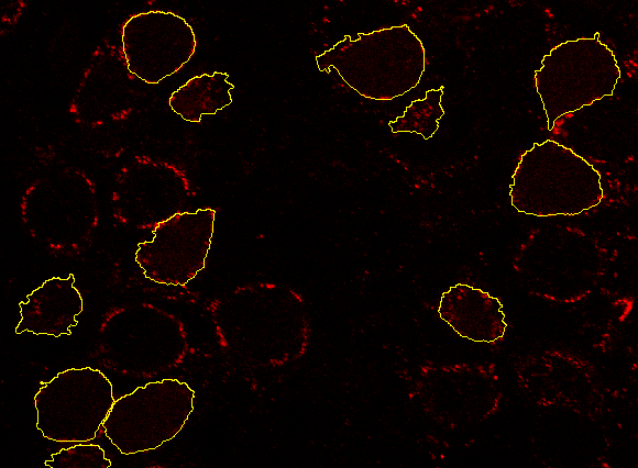
Figure 542. Resulting ROIs.
We will now use the ROIs from the previous step for the final protein count. We click the Add ROI Mask tool and select Inside which we want to measure (Combined). Now we define which features to measure (Count of Cy3 channel in our case). When done we click the button and view the results.
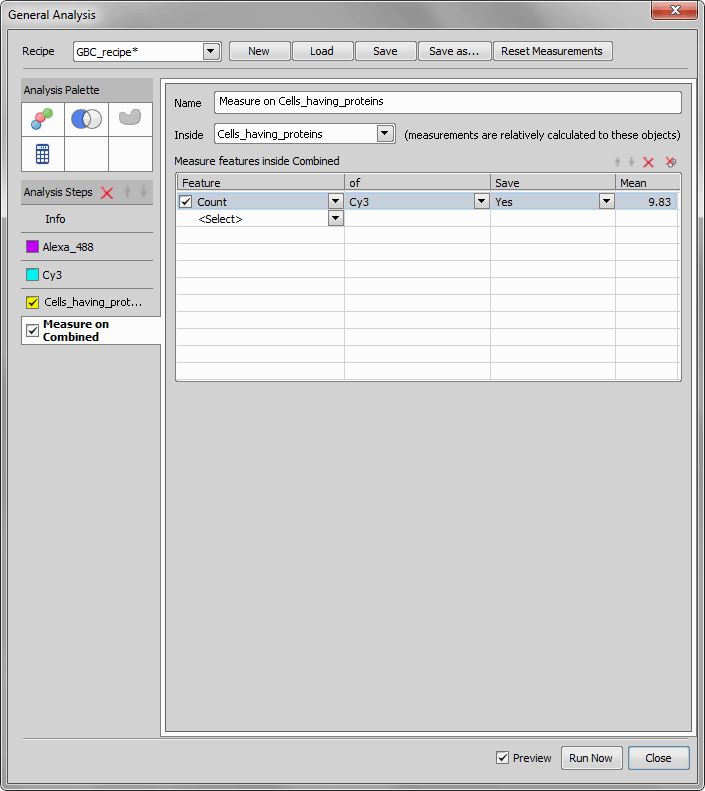
Figure 543. ROI Mask measurement.
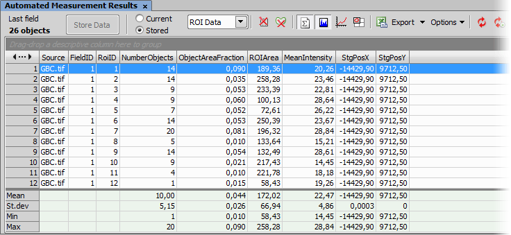
Figure 544. Final results.
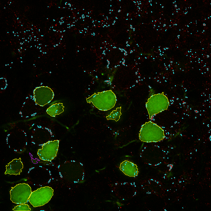
Figure 545. Result visualisation.
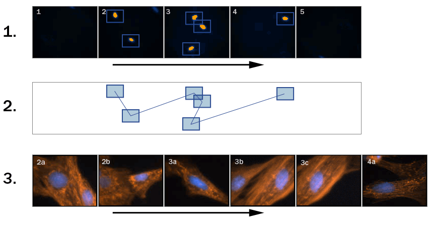
Figure 546. Scheme: GA creates global point set
The slide is scanned at 20x magnification.
General Analysis is used to detect objects and create a new point set with only the objects of interest (their centers).
The new point set is scanned at 40x magnification.
Such a procedure can be carried out using the following tasks.
Scan area
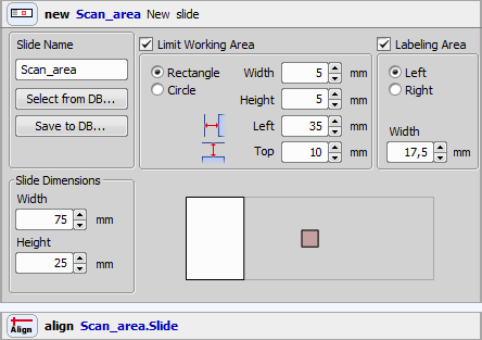
Figure 547.
We are using a 75x25 mm slide with a labeled sticker. We will scan an area of 5x5 mm. The slide must be aligned before the scan begins.
The Detection and the Capturing Point Sets
Figure 548.
There are two point sets in the job. The first point set is to be used with the low magnification objective to detect cell nuclei. The other is an empty point set which will be filled with points based on the General Analysis results.
Capture Definitions
Figure 549.
The first capture definition is used for detection of cell nuclei while the second definition is used to capture two-channel images (nuclei and mitochondria).
Detection Point Loop
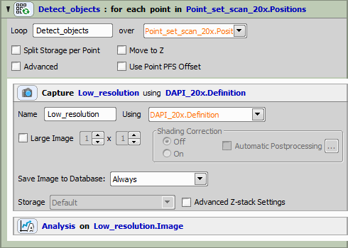
Figure 550.
In the detection point loop, general analysis task is defined, containing two channels (operations):
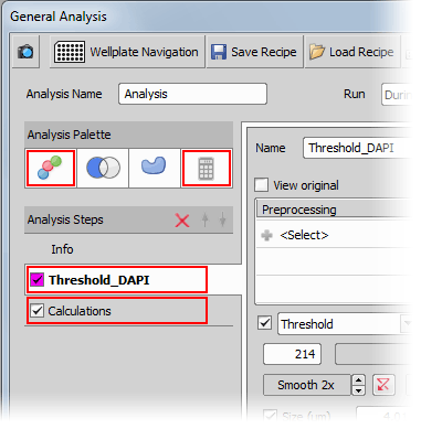
Figure 551. General Analysis Window
Segmentation of the DAPI channel - if an object is detected, its center is appended to the new point set.
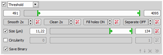
Figure 552. Settings of the Threshold_DAPI channel
New Point Set definition - defines where to store the detected points and that we want to append (not replace) each point.
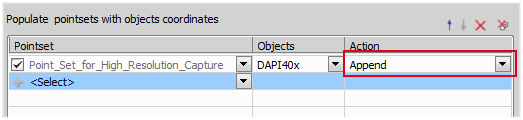
Figure 553. Settings of the Calculations channel - the point set definition
Capturing Point Loop
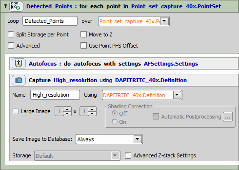
Figure 554. The point loop responsible for high magnification image capturing
The resulting job should look like this:
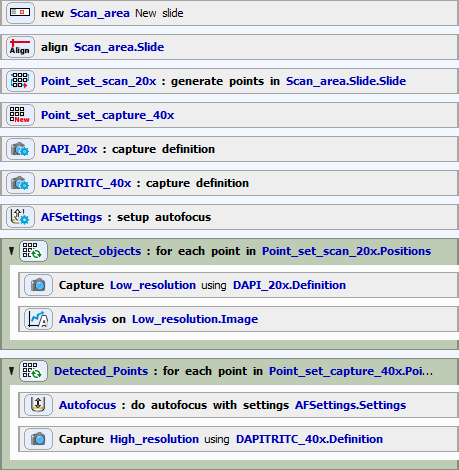
Figure 555. Job Definition
Once the job is started, a progress window appears:
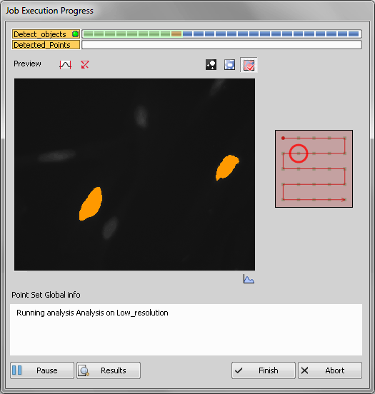
Figure 556. Low resolution capture on DAPI, detection of objects
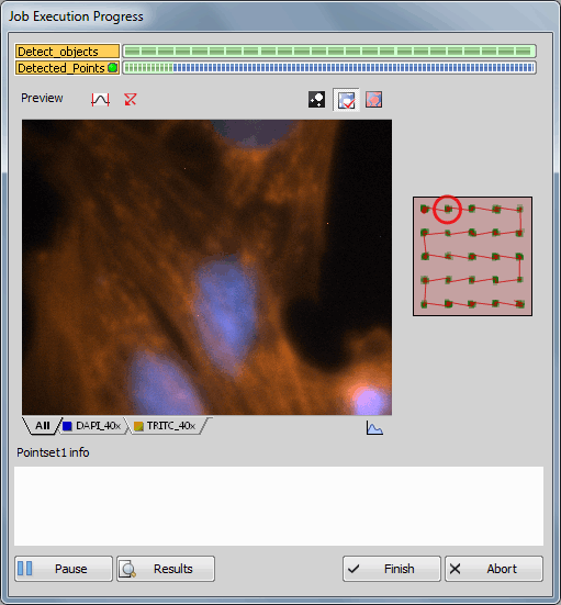
Figure 557. High resolution capture - both image channels
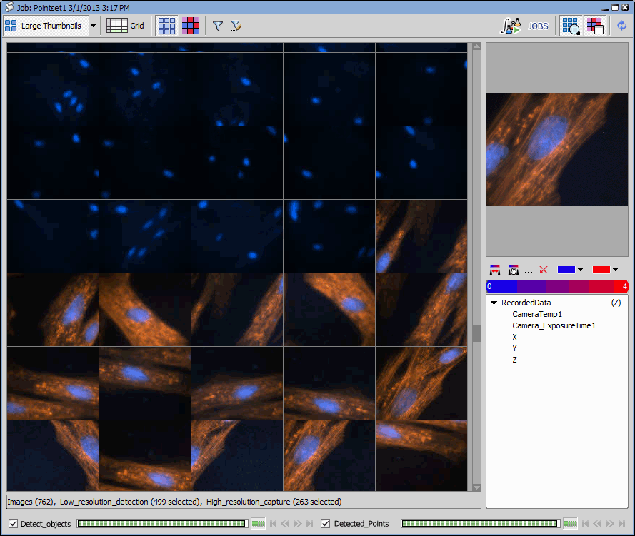
Figure 558. Job Results
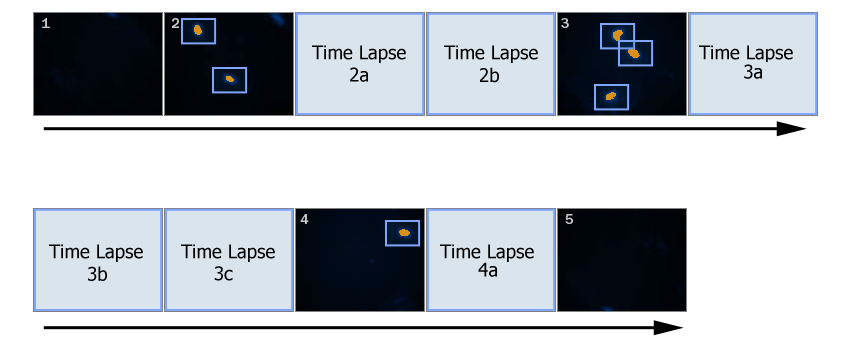
Figure 559. Scheme: GA creates local point set
In this example, unlike in the previous one (General Analysis in JOBS Module - Appended Point Set Use Case), if General Analysis detects one or more objects, a local point set is created and scanned immediately (see Figure 559, “Scheme: GA creates local point set”). Such setup can be used to acquire for example live processes. All time-consuming actions such as objective changing shall be removed in such cases:
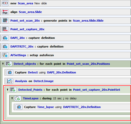
Figure 560.
Tasks arrangement
If you compare this job with the previous one, the biggest difference is in the placement of the Detected_Points point loop which is placed INSIDE of the Detect_objects loop. Furthermore, a time loop has been added.
Detection Point Loop
In the detection point loop, general analysis is defined, containing two channels (operations):
Figure 561. General Analysis Window
Segmentation - if an object is detected, its center is appended to the local point set.
Local Point Set definition - defines where to store the detected points and that we want to run in “replace” mode.
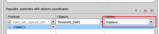
Figure 562. GA: Settings of the Calculation channel