
A histogram is a graphical representation of pixel intensity distribution in the image. It is a basic tool which is used during all phases of an experiment to assess the image information. It is especially useful to make sure there are not too many over- or under-saturated (overrun) pixels. Run the  View > Visualization Controls > Histogram
  command to display the histogram control panel:
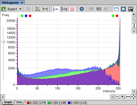
Figure 187.
Source data of the histogram can be viewed if you swap to the Data tab in the bottom-left corner of the window. The area from where the histogram is calculated can be restricted according to the selected histogram mode:

The data are obtained from the whole image.

The data are obtained from within the probe.

The data are obtained from within the current ROI.

The data are obtained from the image parts under the binary layer.
 The source data or the histogram image can be exported to an external file. Display the Export pull-down menu and select a suitable destination. Click the button to perform the export. The Export ND histogram
  button exports histogram data of all frames of the current ND2 file. The same destination which is selected in the Export pull-down menu is applied.
Note
Please, see the Exporting Results chapter for further details.
The histogram can be zoomed in and out using the zoom buttons on sides of the window. There are also other options to adjust the graph appearance:
There is a slider along the Frequency axis. Drag it in order to stretch the view of either lower or upper values of the axis.
 Autoscale All Channels
 Zooms the graph of each channel separately to fit the available area. When this function is ON, the histogram is not proportional.
 Horizontal Auto Scale
 Zooms the graph so that the marginal zero frequencies, if there are some, are excluded from display.
 Graph Linear
 Displays the linear scale on the Y axis.
 Graph Logarithmic
 Displays logarithmic scale on the Y axis.
 Show Grid
 Turns on/off the grid in the background.
If certain amount of pixels with maximum/minimum intensity values (black/white pixels) are spotted in the image, color dots appears above the graph. The color indicates which channel is affected. When you place the mouse cursor over the dots, a tool tip message appears with details about the percentage of under/overexposed pixels. The percentage limit setting is loaded from the LUTs settings (the color dots do not appear unless the set percentage of black/white pixels is exceeded).
Note
If the overrun concerns more than three channels (considering multi-channel images), only one white dot is displayed instead of many color dots.
You can save the current graph to memory and display it later for comparison with another graph.

Displays memorized graph.

Memorizes the current graph. Only one graph can be memorized at a time. If any graph has already been memorized before, it will be overwritten by the current graph.

Clears the memory.
Drawing Style
There are two ways the histogram can be drawn:
Histogram Options Window
The graph appearance can be modified. Press the  button - a window appears where the following settings can be adjusted:
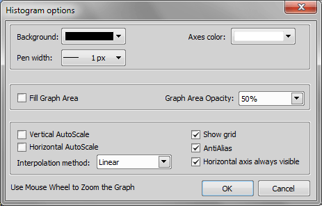
Figure 188. Histogram options window
Graph background and axes colors can be selected.
Set the width of the histogram(s) line to 1, 2, or 3 pixels.
The area below the histogram line can be filled with the channel color.
Select the opacity of the Graph Area color in %.
These options equals the corresponding buttons of the histogram toolbar.
Select the way of drawing the graph line. The Linear (smooth) and Quick (precise) options are available.
Shows the grid of the graph.
Smooths the edges of the graph line.
If checked, the axis does not leave the graph area while zooming in the graph.
If you work with RGB images, you can decide whether to perform the processing on single RGB channels of the image, or on the intensity component of the HSI color representation. The RGB/Intensity setting is global so it is applied to all the other processing commands automatically. When processing a multichannel image, this option is disabled - the operation is applied to channels automatically.
Note
In case the command does not open a window where it would be possible to make the choice, the setting from the last performed processing command (the global setting) is applied.
In image processing, a matrix, also known as a kernel or a filter, is a small rectangular or square grid which acts as a template that slides over the image, and at each position, it interacts with the neighboring pixels to produce a new value for the pixel in the output image. The size of the matrix, also referred to as the kernel size, determines the extent of the neighborhood considered for the computation.
You can select different matrix shapes in some image processing functions which will affect the resulting image. E.g.: Image > Smooth  .
.
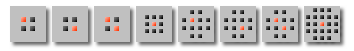
Figure 189. Different matrix shapes
Some functions support a “circular” matrix where different distances from the central pixel are compensated. This is indicated by a circle in the icon.

Figure 190. Circular matrix
E.g.: Binary > Morpho Separate Objects  .
.