
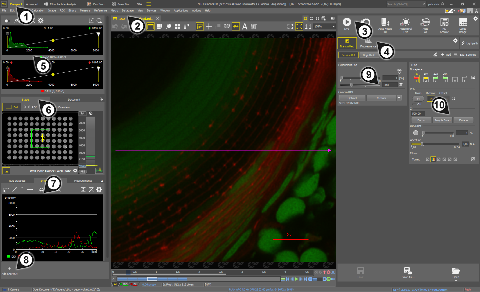
Figure 28. NIS-Elements Compact Layout
Tabs for switching between the layouts.
Opened images displayed as tabs. Each image has its own tool bar. See Image Window.
The
 Acquisition
  panel.
The panel for switching of hardware settings, also called lightpaths. Control panels of devices active in the selected lightpath are displayed below. See
Acquisition Panel.LUTs control panel (
LUTs).Sample navigation panel (Sample navigation).
ROI Statistics, Intensity Profile and Measurements analysis panels (Analysis Panels).
Customizable shortcuts to advanced functions.
Camera and Illumination control panel.
Microscope control pad. (Microscopes).
 Menu
MenuClick  right mouse button on the Compact tab to display a menu with the following options:
See Modifying Layouts.
This panel is used to quickly modify color and brightness of the image using Look-Up Tables (LUTs). Simply drag the left or the right triangle to adjust the input intensity range. Lift or drop the yellow point to adjust the Gamma parameter. Double-click into the graph area to zoom the histogram so that the “high” and “low” limits are distinguishable. For more details about LUTs, please see LUTs - Non-destructive Image Enhancement.
 Keep Auto LUTs
 Auto LUTs
 This button adjusts the white slider position of all channels automatically with the purpose to enhance the image reasonably.
 Reset LUTs
 Settings
 Opens the Auto Scale Settings where the Low and High fields determine how many of all pixels of the picture are left outside the sliders when Auto LUTs are applied (0-10%). Check Use Black Level to ensure that the black slider is influenced by the auto scale functions.
 Pixel saturation indication
 In Color / Mono
 Zoom
ZoomThis panel shows statistics - Mean (Min, Max) - for the drawn ROI.
 Draw Rectangle
 Click and drag in the image to draw a rectangular ROI. To move the ROI, click on its center and move it around. Drag its edge to resize it.
 Draw Circle
 Click and drag in the image to draw a circular ROI. To move the ROI, click on its center and move it around. Drag its edge to resize it.
 Draw Polygon
 Click points in the image to define the polygonal ROI. Use the secondary mouse button or a double-click to place the last node of the polygon and close the object. To draw a free-hand shape, hold down the primary mouse button. To move the ROI, click on its center and move it around.
 Reset
Reset Measure
 Measures the intensity of the whole image or inside the drawn ROI(s) on the selected channel and shows the measured data in the table above. The intensity measurement against the image dimension (Z-Stack, Timelapse) is displayed in the graph below. Select the measured channel from the drop-down menu on the left.
This panel is used for interactive intensity measurements. An arrow is shown in the image indicating the profile cross section. This cross section intensity is shown in the graph. The profile line can be resized by dragging its ends by mouse arbitrarily. It is always a straight line. Context menu over the arrow allows you to Reverse Direction of the arrow, edit Line Properties (color, width and style), change the Intensity Profile Properties (described below) and to choose which channel is used for the measurement.
Click into the graph to define the maximum.
Click again into the graph to define the minimum.
Half of this interval defines the value in which the graph width will be measured.
 FWHM
FWHM This tool measures the Full Width at Half Maximum (FWHM) value on the given graph range.
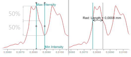
Figure 29.
Note
If the minimum is defined in a different part of graph (e.g.: different peak), the width is measured on the peak where the maximum value was defined.
 Auto FWHM
 Realtime Auto FWHM
 Vertical Autoscale
 Reset
ResetThis panel enables the user to perform simple measurements on the current image.
 Pointing Tool
 Simple Line
 Line length is measured. Click and hold the primary mouse button over the starting position and drag to the ending position and release the button. Confirm the object by the secondary mouse click.
 Polyline
 Polyline length is measured. A polyline consists of several line segments. Use the primary mouse button to draw the line segments. Each mouse-click creates a new node. Complete the total length definition by the clicking the secondary mouse button.
Polygon EqDiameter of a polygon is measured. Draw a polygon by clicking the primary mouse button inside the image. The secondary mouse button or a double-click will place the last node of the polygon and close the object. To draw a free-hand shape, hold down the primary mouse button. Confirm the object by the secondary mouse click.
 Autodetect Polygon
 EqDiameter of a detected object is measured. The system automatically detects a homogeneous area around the clicked point.
 Count
Count Clear Overlay
 Export Data
Shortcuts
Create custom shortcuts to menu commands, macro commands or macro files. The shortcuts pad is closely described here: View > Shortcuts > Create New Shortcuts Pad  .
.
This panel gathers acquisition and hardware control.
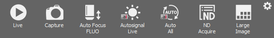
Figure 30.
A431
BSC_1
CHOK_1
Cos7
Day1_iPS_neuro
Day4_iPS_neuro
Day7_iPS_neuro
Hela
HepG2
HT29 J774_1
Neuro2a
 Live
Live Displays the live camera image according to the camera settings (the button changes to Freeze when the live image is shown).
The Smart Live function can be enabled in the  Configure... menu. It works only on Fluorescence experiments. It checks the hardware status, including stage movement and changes in the light power. Then it captures all channels if a hardware change affecting all channels has been made beforehand, such as a movement in XY or Z. However, if a change affecting only one channel has been made (e.g., a change in the power of the associated laser line), the other channels remain unchanged. Once the experiment channel(s) are captured, the light is deactivated. This ensures the convenient access to a multichannel live image without causing bleaching to the sample.
 Auto Focus
 Performs the fastest possible auto focus. There are two focus ranges available, short and long. By default, the short range is used. Hold the Shift key and click on the Auto Focus button to use the long range ( ).
).
The criterion for focus detection is dynamically changed based on the selected light path (modality).
Suitable for brightfield samples. Brightfield auto focus works based on the values set in  Devices > Service Settings
  .
.
Cells.ai Criterion An AI-based algorithm suitable for brightfield cell samples. A specific hardware configuration must be active for this criterion to be available. To switch between the brightfield criterions, use the context menu over the Auto Focus button. The Enable Context Menus option must be selected in the Configure... menu.
The AI neural network has been trained and is intended to be used with the following cell lines:
Note
The Z lens piezo in the system functions with the auto focus only when the register key (HKEY_LOCAL_MACHINE\SOFTWARE\Laboratory Imaging\Misc\DeviceManagerv2\NosepiecePositionForObjectivePiezo) indicates the nosepiece position where the lens piezo is installed and when it aligns with the current nosepiece position. Please create the registry key “NosepiecePositionForObjectivePiezo” as “DWORD(32bit)”. Set the value in hexadecimal, Position #1 = “0”, Position #2 = “1” ... Position #6 = “5”.
 Autosignal
 Automatically finds the optimal camera exposure and light power using an AI algorithm. For brightfield the function adjusts acquisition parameters to utilize the full dynamic range of the camera. For Fluorescence the function adjusts parameters to achieve the required image quality by prioritizing the Signal-to-Noise Ratio (SNR). This SNR-based optimization requires a supported GPU. If a supported GPU is not detected, a warning will be displayed once after clicking the Autosignal button, and the system will fall back to behavior utilizing the full dynamic range.
Autosignal.ai has two options for different algorithm strategies:
To switch between Live Sample and Fixed Sample algorithm, go to the Configure... menu.
 Deshading
 (requires: Local Option)
Turns on the shading correction. The / button appears in the experiment area. Click on the arrow to switch between these two modes and then click on the button itself to define the shading. The definitions are also available in the context menu over the button from where you can open the Shading Correction Panel (Shading Correction with the Local Option module).
 Distortion Correction
 (requires: Local Option)
This function is applied on large images only where it corrects the geometrical image distortion to eliminate duplicated structures in overlapping image tiles. It is closely described in Distortion Correction.ai. Click on the arrow next to the icon to Calibrate Distortion Correction.ai or click  Distortion Correction.ai for information on how to adjust the live image for the large image acquisition and proper distortion correction.
 Auto All
  ND Acquire
 Opens the standard ND Acquisition window (Combined ND Acquisition).
 Large Image
 Runs the Addons > Large Images > Scanning Wizard  command used for a step-by-step large image acquisition.
 Save
Save Save As...
 Open
OpenSee Cameras.
See Illumination Devices.
See Other Devices.
Each opened image is shown as a tab. Click on the tab to activate the image or click X to close it.
The navigation tools at the bottom of the image are the same for both layouts and are described here: Control Bar. The top toolbar buttons are described here.
 Undo
Undo Redo
Redo Auto Calibrate
 Run the live image and click this button to automatically calibrate your image using the current hardware setup.
 Mouse XY
 This feature requires a motorized XY stage. If turned on, the mouse cursor on a live image changes and you can control the XY stage by dragging the live image. Before using this function, it is recommended to perform automatic calibration.
 Split Components
 Turns on a special view, where color channels of the image are displayed separately (tiled). This mode is supported in the modes Main View, Slices View and Volume View.
 Main View
 Show Slices View
 This viewing mode displays orthogonal XY, XZ, and YZ projections of the image sequence. It requires a Z or T dimension.
 Volume View
 Show Tiled View
 This view mode displays frames of the selected dimension arranged one next to other. It requires a Z, T or XY dimension. One or two dimensions can be viewed at a time.
 Show Maximum Intensity Projection
 This function analyses all frames of one dimension and picks pixels with the maximum intensity values. These pixels are used in the resulting image. It requires a Z or T dimension.
 Show Scale
 Displays a line scale which can be moved around the image using the mouse. Context menu over the scale enables the user to Burn Scale into the image permanently, move it to the Default Scale Position, Lock Scale Position or adjust Scale Properties ( View > Layers Properties > Scale Properties).
Tip
Use / to show or hide the scale.
 Show Graticule
 Displays a graticule layer over the image for quick and approximate measurements. Graticules behave like adjustable floating rulers. User can simply align a graticule with the measured object and read the distance value. Click on the line and drag it to move the graticule. Context menu over the graticule enables the user to move the graticule to the center (Move to Center) and adjust the Graticule Properties.
Tip
Use the * key shortcut to show or hide the graticule layer.
 Show Binary
 Displays or hides the binary layer in the image.
Tip
Use Ctrl + Up/Down to decrease/increase the binary layer transparency.
 Show ROIs
 Displays/hides any ROIs in the image. The ROI Statistics panel is shown below the LUTs control.
 Show Intensity Profile
 Displays/hides the intensity profile in the image. The Intensity Profile panel is shown on the left.
 Create EDF Focused Document
 Creates a new simple focused image from an ND file. See Extended Depth of Focus.
 Show EDF Anaglyph
 Enables/disables the anaglyph 3D view. New options appear in the toolbar - you can define the position of the first frame (Lowest/Highest), Style (the color combination used for anaglyph image), Effect (Descend into the Screen / Rise from the Screen) and Z-zoom (define the percentage).
 Show EDF 3D Surface View
 Opens the 3D surface view of the image. See Applications > EDF > Show Surface View  .
.
 Show EDF Z-Profile
 Opens the EDF Z-profile panel with the Z-profile graph of the image. See View > Analysis Controls > EDF Z-Profile  .
.
 Show EDF Z-Map
 Creates a new image displaying the EDF Z-map. See Applications > EDF > Show Z-Map Image.
 Compare View
 Arranges the two last viewed images next to each other and turns on their dimension and zoom synchronization. The synchronization can be turned off by clicking  Synchronize Views (described below).
 Full Screen
 Hides all screen elements such as menus, toolbars, etc. and maximizes the image. Only some basic tools for controlling the image stay displayed. Hit Esc to return to the main view.
 Fit to Screen
 Zoom 1:1
 Single Image
 Tile to Columns
 Tile to Rows Synchronize Views
 If turned on, the views of all currently opened images are synchronized (Z position, zoom, etc.). See also Synchronizer.
 Show Tiles