
Commands for creating and editing binary layers are placed in the menu. Basic methods of binary layer creation are:
This is the most common way of creating a binary layer for image analysis purposes. Use the  View > Analysis Controls > Thresholding
  command to specify threshold limits, a binary layer will be created automatically. See Thresholding.
A binary layer can be edited or even created manually using the built-in binary layer editor. To enter it, click Binary > Binary Editor. See Binary Editor.
There are the following buttons at the bottom of the right image toolbar.
 View Overlay
To manage display of multiple binary layers, use the View > Analysis Controls > Binary Layers  control panel. See Managing Binary Layers.
Run the View > Analysis Controls > Binary Layers command to display the following panel.
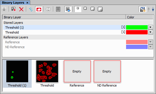
Figure 261.
Each time you create a new binary layer, it is automatically placed into the Working Layers area of the Layer List. Working Layers may be overwritten by the application each time a new binary process is performed. Therefore once you are satisfied with the layer content it is highly recommended to move it into the Stored Layers section using the  Store Current Working Layers.
Binary layers can be selected by mouse (pick more layers holding Ctrl or select a range holding Shift) or you can select all layers by clicking  Select All Layers.
To duplicate one or more binary layers, select them by mouse and drag-drop them to the empty area below the layer list, or click the  button.
Note
If you drag and drop a binary layer to some already existing reference layer, content of the dragged layer is copied to it.
If you drag-drop a binary layer name over another binary layer name, the Binary operations window appears. The same window can be displayed by the  Binary Operations Dialog button.
Note
If multiple layers are selected in the layer list and drag-dropped over another layer, the Binary Operation dialog calculates with multiple (more than two) layers. Available functions are dependent on the number of selected layers.
To create 3D objects in the selected binary layer, click  Connect objects to 3D. If the binary layers are not defined for all frames of the ND document having more than one frame (e.g. only the current frame contains binary information), you can use
  Fill missing binary frames to copy the binary from the current frame to all frames where the binary layer is missing.
Color of a binary layer can be changed using the color pull down menu. It offers a list of predefined colors. Besides the list of predefined colors it is possible to create a custom color (More...) or to colorize objects in a single layer using multiple colors (By Object/By 3D Object).
Use the arrow buttons (
 ) to change the order of the layers in the list.
If a binary layer is created by thresholding in the mode, such binary layer is automatically attached to the channel on which it has been created. Other binary layers can be attached to a channel manually:
Visibility of binary layers attached to channels can be synchronized with channels. Turn ON the
 Synchronize binaries with channels button. Now if a single channel is selected for display, only binary layers attached to it are displayed and vice versa.
To make an attached binary layer global again, right click the binary layer name or thumbnail and select Detach from Component.
The binary layer, as a result of thresholding, can be modified by hand using the binary layer editor. It is a built-in application providing various drawing tools and morphology commands. Go for the Binary > Binary Editor command or press Tab. New buttons appear on the toolbars:
 Undo
Undo Reverses the changes made to the binary image.
 Clear
Clear Clears the binary image (fills the entire image with the “background” color).
 Save
Save Temporarily saves the current binary image. It can be loaded anytime before the binary editor is closed by the Load button.
 Help
Help Displays this help page.
 Exit Editor
 Stores the changes and quits the editor.
The other buttons of the horizontal toolbar are simplified versions of mathematical morphology functions:
 Dilate
  Erode
Erode  Close
Close  Open
Open  Separate Objects
  Clean Fill Holes
  Contour
  Remove Object
 Click this button and then click on a binary object to delete it. Press Esc to finish the deleting.
Erases all binary objects
Please see the Mathematical Morphology Basics chapter.
The binary image can be modified using various drawing tools. Although the way of use of some tools differs, there are some general principles:
Make sure you are in the right drawing mode (drawing background
 /foreground
  )
)Drawing of any object which has not been completed yet can be canceled by pressing Esc.
The polygon-like shapes are drawn by clicks of the primary mouse button. The right button finishes the shape.
The automatic drawing tools (threshold, auto detect) have a changeable parameter. It can be modified by + and - keys or by mouse wheel.
The scene can be magnified by the UP/DOWN arrows when mouse wheel serves another purposes.
You can drag a magnified image by right mouse button.
A line width can be set in the top toolbar.
Hints are displayed in the second top toolbar.
Drawing Tools
 Hand Ctrl+W
 Bezier Hollow N-pt Ctrl+F11
 The object is defined by placing points on its perimeter. The lines connecting those points can vary from straight lines to Bezier curves. (Use +,- keys to adjust them). To finish creation press the right mouse button.
 Bezier Fill N-pt Ctrl+F12
 Polygon Fill F4
 Draws a filled polygon. While holding the primary mouse button down, you are in the free hand mode. When you release it, each click defines a corner of the polygon. The polygon is enclosed and filled by pressing the right mouse button.
 Polygon Hollow F3
 Draws a polygon. It equals the Filled polygon tool, but the resulting object is not filled.
 Circle Fill F8
 Draws a filled circle. Click to determine the center and define the perimeter holding the primary mouse button down.
 Circle Hollow F7
 Draws a circle. Click to determine the center and define the perimeter holding the primary mouse button down.
 Circle 3 Pts. Fill Ctrl+F8
 Circle 3 Pts. Hollow Ctrl+F7
 Rectangle Fill F10
 Rectangle Hollow F9
 Ellipse Fill F12
 Draws a filled movable circle/ellipse. If you grab the ellipse by the center, you can move it. If you grab it by the border, the nearest semi-axis is being modified. When holding down either the SHIFT or the CTRL key, both semi-axes change equally (forming a circle).
 Ellipse Hollow F11
 Freehand pen F1
 Line
Line Polyline
 Auto Detect
 The Auto Detect filled tool. Detect hollows using threshold techniques. Click to the image to place the probe, the detected area is drawn. You can adjust the thresholding range by using the mouse wheel or by pressing the +, - keys.
 Threshold
 Threshold tool. Click into the image to place the probe (or more of them) to define the initial color level for thresholding. Press +,- keys or use the mouse wheel to change the thresholding range.
 FloodFill F6
 Accepted Area Ctrl+F2
 Insert Text
The last button in the left toolbar displays the currently selected tool. You can invoke a pop up menu and select one of the additional commands:
 Auto Detect Hollow B
 The Auto Detect hollow tool. Detect hollows using threshold techniques. Click to the image to place the probe, the hollow is drawn. You can adjust the thresholding range by using the primary mouse button or by pressing the +, - keys.
 Double Cross Ctrl+F1
 Draws rectangularly crossed lines.
 Rose Q
 Draws a rose. Click to the image to define the center, than drag the mouse to set the length of it's arms.
 Markers
 Places a marker to the image. Simply click into image...
 Select objects
 Selects binary objects.
 Connect
 The Connect tool. Draws a line(s) from the place you've clicked to the nearest object(s).
 Show Grid
 Displays a grid. Visible only when using magnification 400% and higher.
 Hide Overlay
 Hides the overlay.
 Smooth
 See the Mathematical Morphology Basics chapter.
Contour See the Mathematical Morphology Basics chapter.
 Inversion
 Inverts the binary image. Foreground becomes background and vice versa.
When in overlay mode:
The Insert key switches between predefined overlay colors.
Ctrl + Up/Down increases/decreases the binary layer transparency.
Single binary objects can be erased in the following way:
Click inside the objects to be erased.
An arbitrary number of binary layers can be created within one image. Click this Create New Binary Layer  button in the image toolbar to add a new binary layer. The binary layer that you are currently editing can be selected in the nearby pull-down menu. Binary layers can be managed from the View > Analysis Controls > Binary Layers control panel.
The binary image as a result of thresholding often needs to be modified before a measurement is performed. Edges of the objects can be smoothed, holes in the objects filled, etc. by using the mathematical morphology commands.
Note
“Image Analysis and Mathematical Morphology” by J. Serra (Academic Press, London, 1982) was used as a reference publication for the following overview.
The following tools perform basic morphology operations. You can find them in the Binary menu or in the View > Analysis Controls > Binary Toolbar  panel.
Erode After performing erosion, the objects shrink. Marginal pixels of the objects are subtracted. If an object or a narrow shape is thinner than the border to be subtracted, they disappear from the image.
Dilate After performing dilation, the objects enlarge. Pixels are added around the objects. If the distance between two objects is shorter than twice the thickness of the border to be added, these objects will be merged. If a hole is smaller than twice the thickness of the border, it disappears from the image.
Open Open is erosion followed by dilation so the size of the objects is not significantly affected. Contours are smoothed, small objects are suppressed and gently connected, particles are disconnected.
Close Closing is a dilation followed by erosion so the size of objects is not significantly affected. Contours are smoothed, small holes and small depressions are suppressed. Very close objects may be connected together.
Clean This transformation is also called geodesic opening. The image is eroded first so small objects disappear. Then, the remaining eroded objects are reconstructed to their original size and shape. The advantage of this algorithm is that small objects disappear but the rest of the image is not affected.
Homotopic transformations preserve topological relations between objects and holes inside them. Using a homotopic transformation, an object with 5 holes will be transformed to another object with 5 holes. Two objects without any holes, even if they are very near each other, will become again two objects without holes, but likely with a different shape and size. Opening, Closing, Erosion and Dilation are not homotopic transformations. Typical homotopic transformations in NIS-Elements are: Skeletonize, Homotopic Marking and Thickening.
Applying the above mentioned transformations has some limitations due to digital images rasterization.
When speaking about binary image processing, a binary image is a set of pixels where values 1 represent objects and values 0 represent background. In the square grid of the image, two possible connectivities can be used for processing - the 8-connectivity or the 4-connectivity. Look at the picture below. If the 8-connectivity is used, the two pixels represent one object. If the 4-connectivity is applied, there are two objects in the picture. NIS-Elements works with the 8-connectivity model, so all pixels neighboring by the corner belong to one object.

Figure 262.
When applying Erosion, Dilation, Opening or Closing, one of the parameters which determines the transformation result is the selection of kernel (structuring element, matrix) type. There are the following kernels used in NIS-Elements:
Figure 263.
The bright pixel in the center or near the center of the kernel represents its “midpoint”.
Example 2. Erosion
Let's assume 1 and 0 represent object(1) and background(0) pixels of the binary layer. You can imagine the erosion as the following algorithm:
Move the midpoint of the kernel to every point of the image. Each time, look at the neighboring pixels of the kernel and make the following decision:
If there are object(1) pixels in all the positions of the kernel, set the midpoint to object(1).
If there is at least one background(0) pixel in the kernel, set the midpoint to background(0).
Example 3. Dilation
You can imagine the dilation as the following algorithm:
Move the midpoint of the kernel to every point of the image. Each time, look at the neighboring pixels of the kernel and make the following decision:
If there is at least one object(1) pixel in any position of the kernel, set the midpoint to object(1).
If there are background(0) pixels in all the positions of the kernel, set the midpoint to background(0).
Example 4. Open and Close
Open is performed by eroding the image and then applying a dilation to the eroded image. On the contrary, Closing is performed as a dilation followed by erosion.
If the midpoint is not in the center, applying erosions or dilations by odd number of iterations causes image to shift by 1 pixel. Normally, the total image shift would be determined by the number of Iterations (in pixels). NIS-Elements eliminates this shift: it changes the position of the midpoint 1 pixel down-rightwards within the kernel for even operations. For opening and closing it is possible to eliminate this shift totally. However, if you run the erode or dilate processes again and again using the kernel with even dimensions and odd number of iterations, then the shift becomes significant.
Please see the following examples of some of the binary functions applied to an image. In the following sequence of images, the functions were applied subsequently:
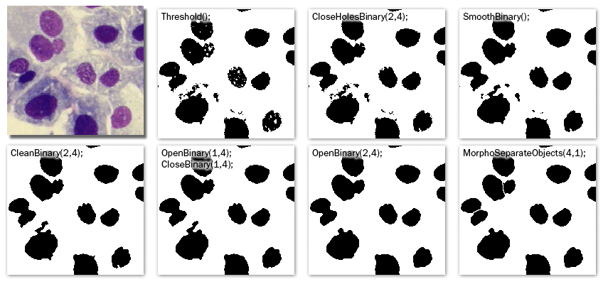
Figure 264. Functions applied subsequently
The following images were created by calling each of the functions separately:
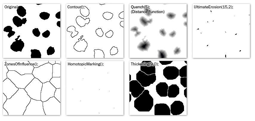
Figure 265. Single function applied to the original
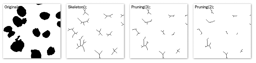
Figure 266. Other functions applied subsequently