
Determines cell viability across a multi-well plate using dual fluorescent staining. Live cells are identified by the presence of Hoechst (nuclear stain) without Ethidium (dead cell marker). This workflow is designed for high-content screening (HCS) applications including cytotoxicity assays, drug screening, and dose-response studies.
This workflow produces:
Segmentation of all cells (Hoechst-positive).
Identification of dead cells (Ethidium-positive).
Calculation of live cells (cells without Ethidium).
Per-well statistics: total cells, live cells, dead cells, and viability ratio.
Dose-response curve fitting with IC50 calculation.
Well-plate visualization: heatmaps, bar charts, and plate layouts.
Statistical quality metrics (Z’ factor).
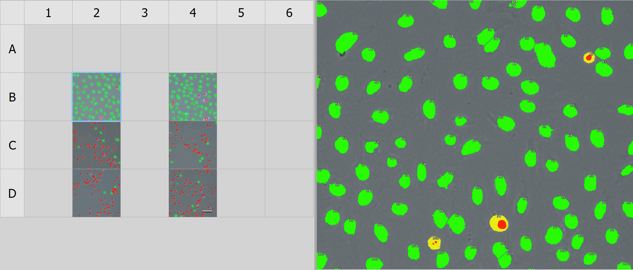
Figure 736.
The recipe consists of:
Dual channel segmentation block.
Live/dead discrimination block.
Well-plate measurement block.
Data aggregation and analysis block.
High-content screening presentation block.
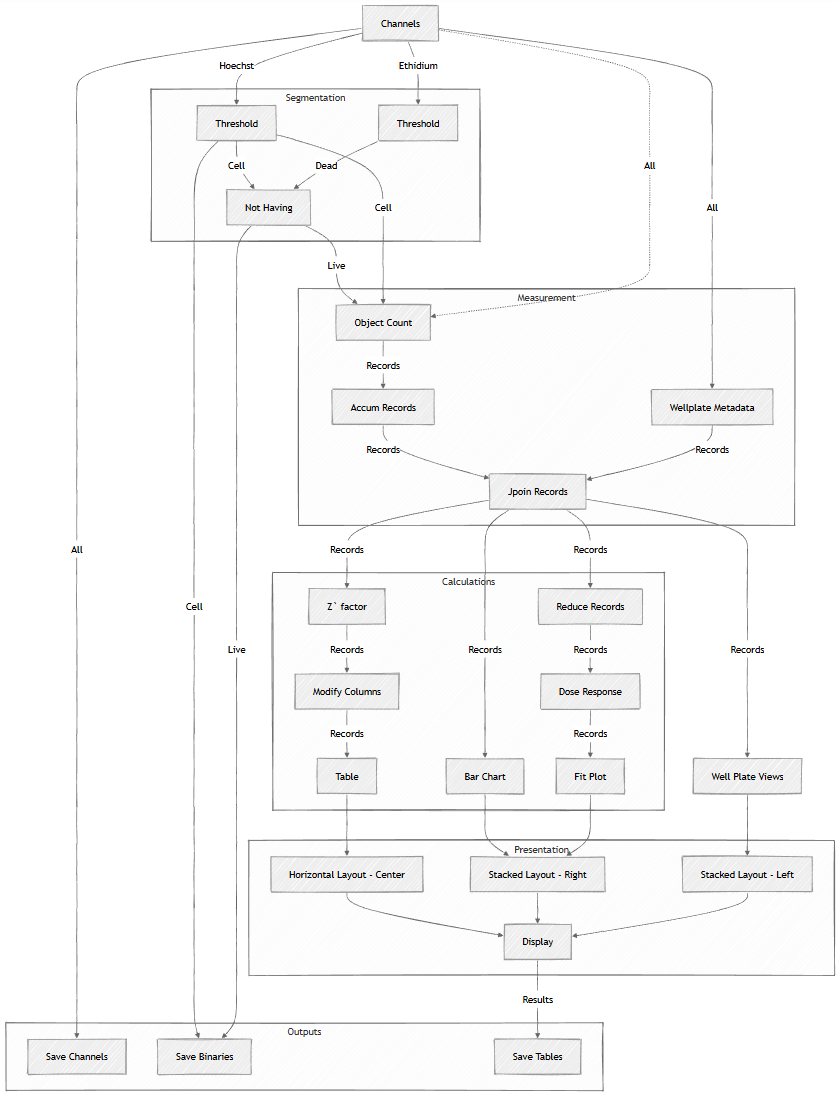
Figure 737. Schematic
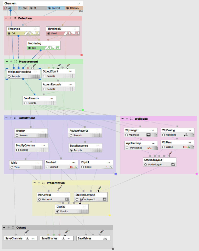
Figure 738. Recipe
Cell detection (Hoechst)
Threshold on the Hoechst channel detects all cell nuclei, which serve as markers for total cell count. Hoechst is a cell-permeable DNA stain that labels nuclei in both live and dead cells.
The node uses:
Auto Threshold Method: Li algorithm for robust nuclear detection.
Clean: 0.63 µm to remove small debris.
Fill: ON to fill all holes.
Separate: 0.315 µm to split touching nuclei.
Smooth: 0.63 µm to regularize boundaries.
IntensityLow: 626 (manual threshold adjustment if needed).
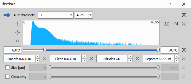
Figure 739.
Note
The Hoechst channel provides the total cell count. It is important to optimize these settings to accurately detect all cells, as this forms the basis for viability calculations.
Dead cell detection (Ethidium)
Threshold on the Ethidium channel identifies dead or membrane-compromised cells. Ethidium homodimer (EthD-1) or similar probes only penetrate damaged cell membranes and bind to DNA, producing strong fluorescence.
The node uses:
Clean: 0 µm (no cleaning, to preserve even weak signals).
Fill: ON to fill all holes.
IntensityLow: 998 (manual threshold for dead cell signal).
The threshold is typically higher for Ethidium because only dead cells should show signal. Setting it too low will produce false positives (live cells incorrectly marked as dead).
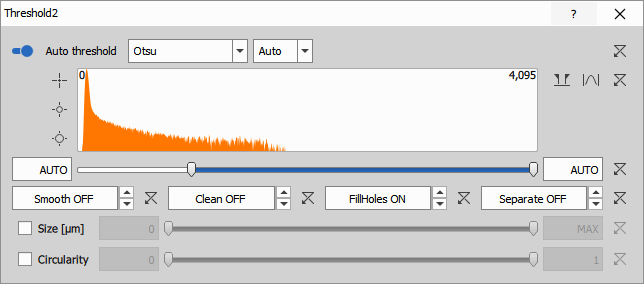
Figure 740.
Note
Critical parameter: The Ethidium threshold (IntensityLow) must be set carefully. Too low will mark healthy cells as dead; too high will miss dying cells. Use the histogram and preview to find the optimal separation between background and true positive signal.
Not Having operation
Binary operations > Binary x Binary > Not Having is a binary operation that identifies cells from the first binary (all cells from Hoechst) that do NOT contain any pixels from the second binary (dead cell markers from Ethidium).
This elegant operation implements the live cell definition:
Input A: All cells (Hoechst-positive nuclei).
Input B: Dead cells (Ethidium-positive nuclei).
Output: Live cells = cells that are Hoechst-positive but Ethidium-negative.
The logic is simple but powerful: if a cell nucleus overlaps with any Ethidium signal, it is classified as dead. Otherwise, it is live.
Note
The Not Having node creates three distinct populations:
All cells (green): From Hoechst threshold.
Dead cells (red): From Ethidium threshold.
Live cells (cyan): Cells not overlapping with Ethidium.
These three layers provide complete visualization of cell viability status.
Object Count with calculated features
Measurement > Basic > Object Count measures field-level statistics for each well. This node can process multiple binary inputs simultaneously to count different populations.
The node measures:
System columns:
Well name and position (A1, A2, B1, etc.).
Well metadata (compound, concentration, control status).
Measured features:
AllCells: Count of all Hoechst-positive nuclei.
LiveCells: Count of cells without Ethidium signal.
DeadCells: Calculated as AllCells - LiveCells.
LiveRatio: Calculated as LiveCells / AllCells.
Calculated columns: These use the calculator feature to derive additional metrics:
DeadCells = AllCells - LiveCells
LiveRatio = LiveCells / AllCells (expressed as 0-1)
The measurements are performed per well, typically with multiple fields (sites) per well that are later aggregated.
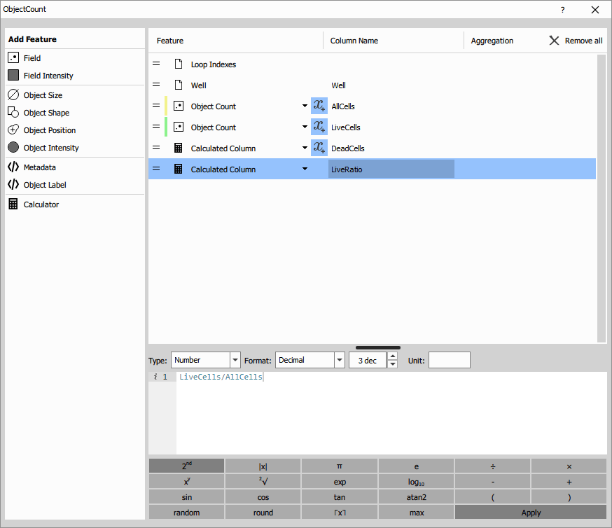
Figure 741.
Reduce Records
Data manipulation > Basic > Reduce Records aggregates multiple fields within each well into a single per-well measurement. For a 96-well plate with 4 fields per well, this reduces 384 records to 96 records.
Aggregation typically uses:
Sum for cell counts (total cells across all fields).
Mean for ratios and percentages.
Standard deviation for quality metrics.
Modify Columns
Data manipulation > Basic > Modify Columns prepares the data for visualization by:
Calculating statistics like Z’ factor for assay quality.
Adding well plate metadata (row, column, compound names).
Formatting columns for display.
Creating thumbnail images of representative fields.
Statistical quality metrics
The Z’ (Z-prime) factor is calculated to assess assay quality:
Z’ = 1 - (3σ_pos + 3σ_neg) / |μ_pos - μ_neg|
Where:
σ_pos, σ_neg = standard deviations of positive and negative controls.
μ_pos, μ_neg = means of positive and negative controls.
Z’ interpretation:
Z’ > 0.5: Excellent assay.
0.5 > Z’ > 0: Acceptable assay.
Z’ < 0: Poor assay (high variability or small signal window).
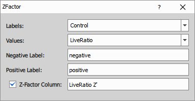
Figure 742.
Dose Response curve fitting
Data manipulation > Curve Fitting > Dose Response fits a dose-response curve to the live ratio data across different compound concentrations. This is essential for IC50 determination in drug screening.
The node uses a 4-parameter logistic model:
Response = Bottom + (Top - Bottom) / (1 + (Dose/IC50)^Hill)
Parameters:
Top: Maximum response (100% viability at zero concentration).
Bottom: Minimum response (0% viability at high concentration).
IC50: Concentration producing 50% effect.
Hill coefficient: Slope of the curve (cooperativity).
Settings:
Model: 4-parameter logistic (default).
Dose column: Concentration from well metadata.
Response column: LiveRatio.
Zero handling: Substitution with 0.1 (for log-scale plotting).
Display: Equation, IC50 value.
The output includes:
Fitted curve parameters for each compound.
IC50 values with confidence intervals.
Goodness of fit (R2).
Predicted values for plotting.
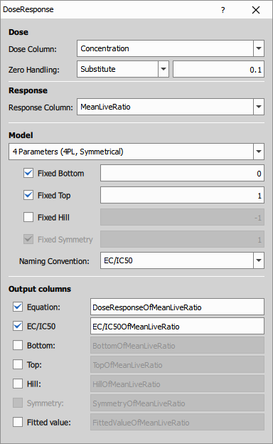
Figure 743.
Note
IC50 naming convention: The node can output different IC50-related values:
IC50: Concentration for 50% inhibition.
EC50: Effective concentration for 50% effect.
GI50: Growth inhibition 50%.
Choose the appropriate terminology for your assay in the node settings.
This workflow uses specialized well-plate visualization nodes designed for HCS data.
Well Plate Image
Results & Graphs > Wellplate > Image displays thumbnail images of each well in the plate layout. This provides a visual overview of the entire experiment and helps identify spatial patterns or artifacts.
Features:
Thumbnail images from representative fields.
Color-coded by experimental conditions.
Interactive selection linking to other views.
Customizable plate dimensions (96, 384, 1536 wells).
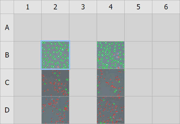
Figure 744.
Well Plate Dosing
Results & Graphs > Wellplate > Dosing visualizes the dosing scheme across the plate. It shows which wells contain which compounds and concentrations, helping verify the experimental design.
Displays:
Compound names per well.
Concentration gradients.
Control well positions.
Replicate patterns.
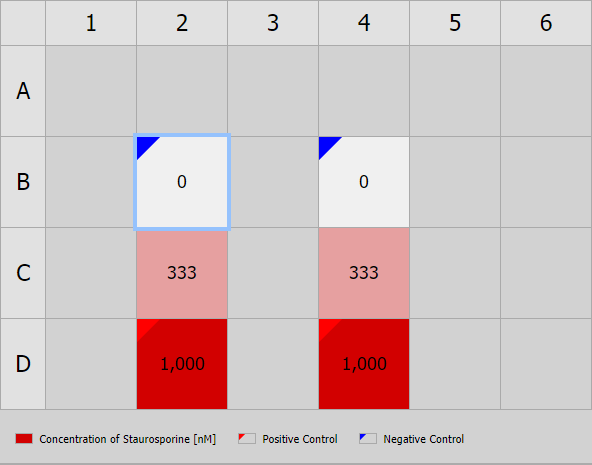
Figure 745.
Well Plate Heatmap
Results & Graphs > Wellplate > Heatmap displays the measured values (e.g., LiveRatio) as a color-coded heatmap in the plate layout.
Features:
Color scale representing measurement values.
Immediate identification of wells with extreme values.
Pattern recognition for edge effects or artifacts.
Multiple color maps available (viridis, RdYlGn, etc.).
This view is excellent for quality control and identifying spatial trends.
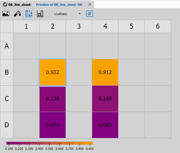
Figure 746.
Well Plate Bars
Results & Graphs > Wellplate > Bars shows bar charts for each well, useful for comparing values across the plate.
Features:
Bar height represents measurement value.
Side-by-side comparison of conditions.
Error bars for replicate measurements.
Interactive selection.
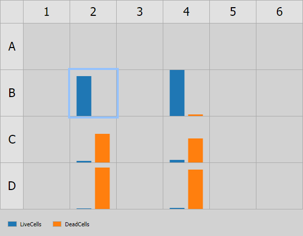
Figure 747.
Results Table
Results & Graphs > Tables > Table displays the per-well statistics in tabular format with:
Display: All data (all wells shown).
Selection: Enabled for linking to plate views.
Sorting: Enabled for ranking by any column.
Statistics: Min, max, mean across all wells.
Columns include:
Well identifier (A1, A2, etc.).
Compound and concentration.
AllCells, LiveCells, DeadCells.
LiveRatio.
Z’ factor.
Thumbnail images.
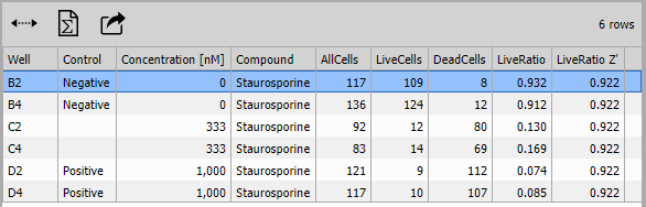
Figure 748.
Bar Chart
Results & Graphs > Graphs > Barchart displays grouped bar charts comparing measurements across conditions (e.g., compounds or concentrations).
Features:
Grouping by compound or concentration.
Multiple series (AllCells, LiveCells, DeadCells).
Error bars for replicates.
Color coding by condition.
This view is ideal for comparing the effects of different treatments.
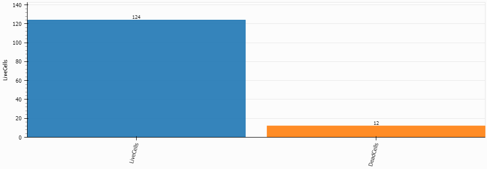
Figure 749.
Fit Plot
Results & Graphs > Graphs > Fitplot displays the dose-response curves fitted by the Data manipulation > Curve Fitting > Dose Response node.itemi
Features:
Fitted curves overlaid on raw data points.
Multiple compounds on the same plot.
Log scale on concentration axis.
IC50 values annotated.
Confidence bands (optional).
Interactive legend.
This is the key result for drug screening experiments, showing the potency of each compound.
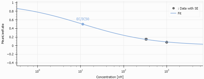
Figure 750.
Layout organization
The presentation uses a three-pane layout created by combining layout nodes:
Left pane (Results & Graphs > Layout > Stacked):
Well Plate Image.
Well Plate Dosing.
Well Plate Heatmap.
Well Plate Bars.
Center pane (Results & Graphs > Layout > Horizontal):
Results Table.
Right pane (Results & Graphs > Layout > Stacked):
Bar Chart (compound comparison).
Fit Plot (dose-response curves).
The Results & Graphs > Layout > Display node combines all three panes into a synchronized interface where:
Selecting a well in any plate view highlights it in all other views.
Selecting a row in the table highlights the well in plate views.
All views update together for seamless data exploration.
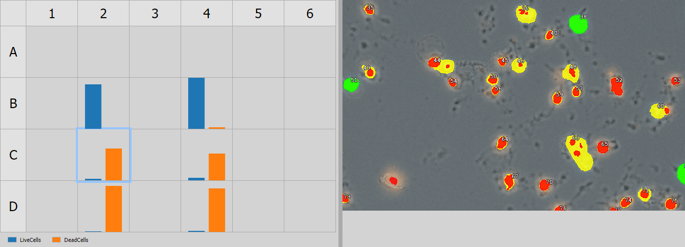
Figure 751.
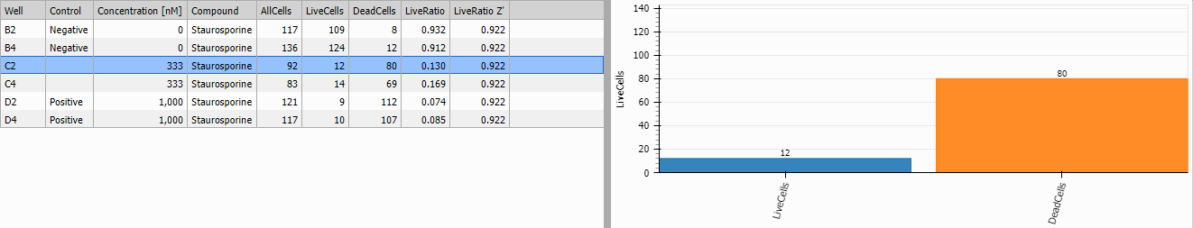
Figure 752.
The recipe saves three types of output:
Save Channels
Input & Output > Save to Document > Save Channels saves the original Hoechst and Ethidium image channels for all wells.
Save Binaries
Input & Output > Save to Document > Save Binaries saves segmentation masks:
Cell binary layer: All detected cells.
Live binary layer: Live cells only.
(Dead cells can be derived by subtracting Live from Cell).
Save Tables
Input & Output > Save to Document > Save Tables saves:
Per-well statistics table.
Dose-response parameters.
Z’ factors and quality metrics.
High false positive rate (live cells marked as dead)
Causes:
Ethidium threshold too low.
Autofluorescence in Ethidium channel.
Phototoxicity from excessive imaging.
Solutions:
Increase Ethidium IntensityLow parameter.
Use background subtraction if autofluorescence is uniform.
Reduce laser power or exposure time.
Image Ethidium channel last.
Low cell counts
Causes:
Cell seeding too low.
Cell death during incubation.
Poor Hoechst staining.
Hoechst threshold too high.
Solutions:
Optimize cell seeding density (5,000-10,000 cells/well for 96-well).
Check cell culture conditions.
Verify Hoechst concentration and incubation time.
Lower the Hoechst threshold (reduce IntensityLow).
Inconsistent results across wells
Causes:
Uneven cell seeding.
Edge effects (evaporation in outer wells).
Pipetting errors in compound addition.
Temperature gradients.
Solutions:
Use multi-channel pipettes or liquid handlers.
Fill outer wells with PBS or media (do not use for measurements).
Verify compound stock concentrations.
Ensure even incubator temperature.
Poor dose-response curves
Causes:
Insufficient concentration range (does not cover IC50).
Too few concentration points.
Wrong concentration units or log transformation.
Outlier wells.
Solutions:
Use at least 8-10 concentrations spanning 3-4 orders of magnitude.
Center the range around expected IC50.
Verify concentration metadata is correct.
Check for outliers and exclude bad wells if justified.
Cells merging or undersegmented
Causes:
Cells too confluent.
Nuclei touching.
Separate parameter too low.
Solutions:
Reduce cell seeding density (aim for 50-70% confluence).
Increase Separate parameter in Threshold.
Consider using watershed-based segmentation for very confluent cultures.
Before running a screening campaign, validate the assay:
Dynamic range: Confirm 0% and 100% controls are well separated.
Reproducibility: Run same plate multiple times, calculate inter-assay CV.
Linearity: Test if response is linear with cell number.
IC50 accuracy: Test reference compounds with known IC50 values.
Z’ factor: Should consistently achieve Z’ > 0.5.
Document these validation results before proceeding to screening.
Results can be exported for further analysis:
Excel format: Per-well statistics and dose-response parameters.
CSV format: Compatible with R, Python, GraphPad Prism.
Images: High-resolution images and segmentation masks.
Metadata: Plate layout, compound information, experimental conditions.