
Extends standard 2D workflows to analyze volumetric (3D) image data typically acquired by confocal scanning or a spinning disk. Light-sheet imaging is becoming common too.
Instead of analyzing individual slices, these workflows process complete Z-stacks as single volumes, detecting and measuring true 3D objects. Although 3D imaging and analysis is much closer to the reality it brings several challenges (3D-specific challenges).
Key differences from 2D:
Dimensionality:
2D: Objects are patches of connected pixels (X, Y).
3D: Objects are volumes of connected voxels (X, Y, Z).
Measurements:
2D: Area, perimeter, circularity (µm2, µm).
3D: Volume, surface area, sphericity (µm3, µm2).
Processing:
2D: Frame-by-frame through time-lapse.
3D: Volume-by-volume through time series.
Visualization:
2D: Single slice or maximum projection.
3D: Volume rendering, Z-projections.
When to use 3D analysis:
Required for:
Spherical or irregular 3D structures (organoids, spheroids, cell clusters).
True volumetric measurements.
3D spatial relationships between objects.
Tracking particles moving in 3D space.
Not necessary for:
Flat monolayer cell cultures.
Objects confined to single focal plane.
When 2D measurements are sufficient (e.g., cell counting).
All three workflows share these 3D-specific components:
3D segmentation nodes
Replace 2D segmentation with volumetric equivalents:
Bright Spots 3D instead of Bright Spots.
Threshold 3D instead of Threshold.
Cellpose 3D instead of Cellpose.
These nodes detect objects across the entire Z-stack simultaneously.
3D measurement nodes
Provide volumetric features:
Object 3D Count - counts objects per volume.
Object 3D Measurement - measures 3D morphology.
Time and Center 3D - extracts 3D centroids.
Processing mode
GA3 automatically switches to volume-by-volume processing when 3D nodes are present. Instead of processing frame 1, frame 2, etc., it processes volume 1, volume 2, etc.
Calibration requirements
3D analysis requires proper Z-calibration:
XY calibration: Microns per pixel (typically 0.1-1 µm/pixel).
Z calibration: Microns per slice (typically 0.2-2 µm/slice).
Incorrect Z-calibration produces distorted measurements (spheres appear as ellipsoids).
Detects and counts 3D objects across time-series volumes, measuring object counts and intensities per volume.
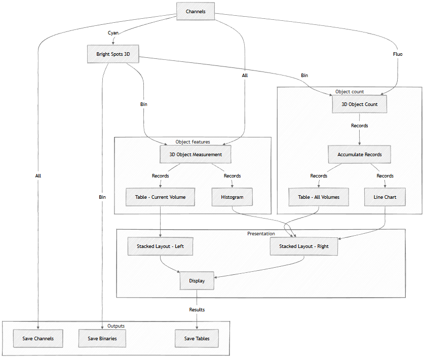
Figure 753. Schematic.
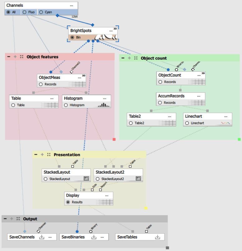
Figure 754. Recipe.
Bright Spots 3D detection
Bright Spots 3D detects fluorescent spots as 3D objects:
Parameters:
Diameter: 8 microns - expected object diameter in XY.
Contrast: 100 - minimum brightness above background.
Z-Axis elongation: 1:2 - typical anisotropy.
Output type: “Centers” - creates centroids for fast rendering but only for counting.
The algorithm searches for local intensity maxima and grows them in 3D until background is reached or growth limits are hit.
Object 3D Count measurement
Object 3D Count provides per-volume statistics:
Measured features:
Time: Timestamp of the volume.
Object Count 3D: Total number of 3D objects in volume.
Mean Intensity: Average intensity per channel (aggregated across objects).
This produces one row per volume (time point), summarizing the entire 3D field.
Object 3D Measurement
Object 3D Measurement measures individual object features:
3D morphological features:
Volume: Object volume in µm3.
Surface Area: Outer surface area in µm2.
Equivalent Diameter: Diameter of sphere with same volume.
Sphericity: How sphere-like the object is (1 = perfect sphere).
Width, Height, Depth: Bounding box dimensions in µm.
Center X, Y, Z: 3D centroid coordinates.
3D intensity features:
Mean, min, max, sum, standard deviation.
Measured in all intensity channels.
Each row represents one 3D object in one volume.
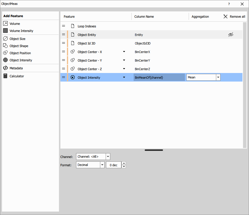
Figure 755.
Accumulate Records
Data manipulation > Basic > Accumulate Records collects object counts across all volumes:
Tracks count evolution over time.
Enables temporal analysis.
Visualization
Shows features of all objects in the currently displayed volume.
Displays object counts and statistics for all volumes.
Plots object count vs. time, showing population dynamics.
Displays distribution of selected feature (e.g., volume, sphericity) for current volume objects.
Results
This workflow produces:
Per-volume object counts over time.
Individual 3D object measurements (volume, shape, intensity).
Temporal trends in object population.
Feature distributions.
Use cases
Organoid counting, spheroid growth analysis, 3D spot quantification, vesicle counting in volumes.
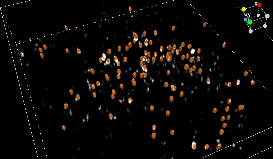
Figure 756.
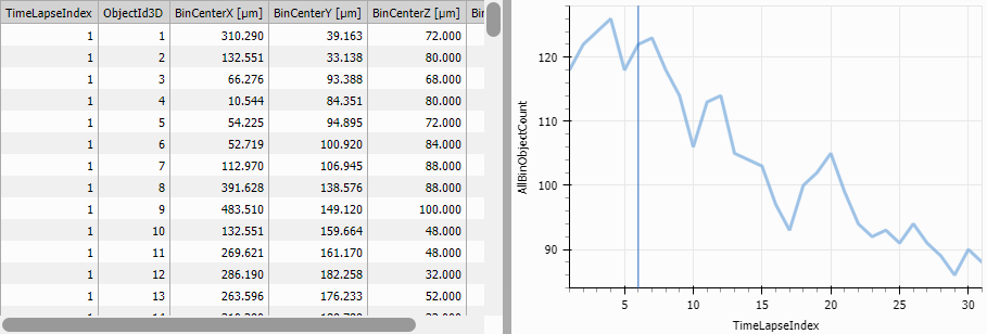
Figure 757.
Tracks particles moving in 3D space, calculating motion features including 3D trajectories and velocities.
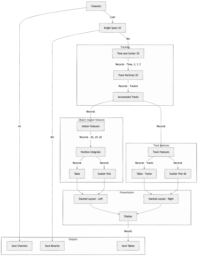
Figure 758. Schematic.
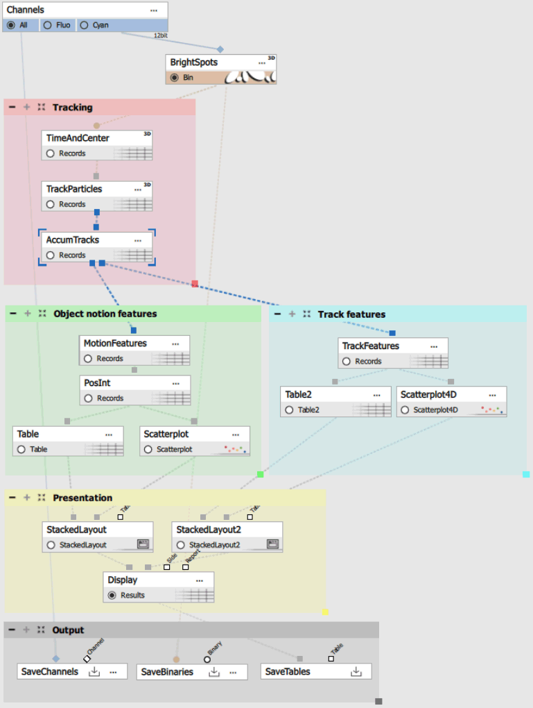
Figure 759. Recipe.
Time and Center 3D
Tracking > Object Position > Time & Center ![]() extracts 3D positions:
extracts 3D positions:
Measured features:
Time: Timestamp.
CenterX, CenterY, CenterZ: 3D centroid coordinates.
Provides the position data needed for 3D tracking.
Track Particles 3D
Tracking > Tracking > Track Particles ![]() connects particles across volumes in 3D space:
connects particles across volumes in 3D space:
Parameters:
maxSpeed: 146 µm/volume - maximum 3D displacement between volumes.
maxGap: 2 volumes - allows temporary disappearance.
Algorithm: Calculates 3D Euclidean distance between particle positions:
distance = sqrt((x₂-x₁)² + (y₂-y₁)² + (z₂-z₁)²)
Particles within maxSpeed distance are candidates for linking. The algorithm chooses the globally optimal assignment.
Note
3D tracking considerations:
Z-resolution is typically coarser than XY (0.5 µm vs 0.1 µm).
Particles may move out of the imaged volume.
Acquisition time per volume is longer (slower temporal resolution).
Set maxSpeed accounting for 3D movement including Z-displacement.
Accumulate Tracks 3D
Tracking > Tracks > Accumulate Tracks collects tracks with:
MinSegmentCount: 5 volumes minimum.
Filters out short, unreliable 3D tracks.
Motion Features 3D
Tracking > Tracking Features > Tracking Features > Motion Features calculates 3D motion parameters:
3D motion features:
Speed: 3D velocity magnitude (µm/s).
Direction: 3D heading (azimuth and elevation angles).
dPositionX, dPositionY, dPositionZ: Displacement components.
Acceleration: Rate of 3D speed change.
These capture full 3D motion dynamics.
Track Features 3D
Tracking > Tracking Features > Track Features summarizes entire 3D trajectories:
Per-track features:
Length: Total 3D path length traveled.
Duration: Time span.
Speed: Mean 3D speed.
LineLength: Straight-line 3D distance start to end.
Straightness: LineLength / Length.
Position Integration
Sequential Data manipulation > Sequences > Position Integrate reconstructs 3D trajectories by integrating displacement vectors:
Starting from an arbitrary origin, adds each displacement:
Position(t) = Position(t-1) + [dX, dY, dZ]
This creates smooth 3D trajectories suitable for visualization.
3D trajectory visualization
Projects 3D trajectories onto the XY plane, color-coded by track. Shows spatial distribution and horizontal movement patterns.
Displays tracks in multidimensional feature space (e.g., speed vs. length vs. straightness), enabling population analysis.
Show per-volume positions and per-track summaries.
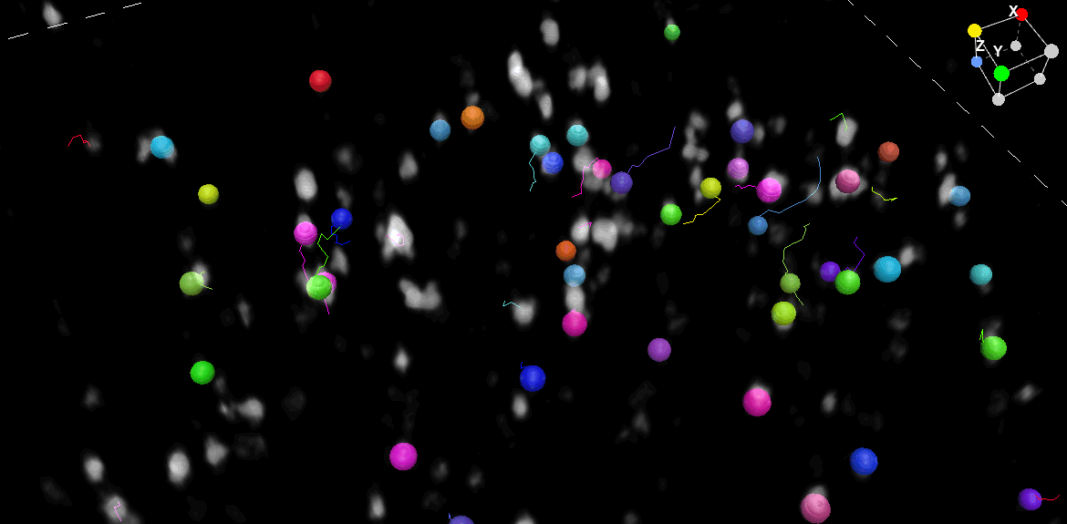
Figure 760.
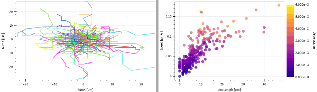
Figure 761.
Results
This workflow produces:
3D track IDs linking particles across volumes.
Complete 3D trajectories (X, Y, Z, time).
3D motion features (speed, direction, acceleration in 3D).
Track statistics (3D path length, 3D displacement).
Use cases
Vesicle trafficking in 3D, organelle movement, intracellular particle transport, cell migration in 3D matrices.
Measures morphology and intensity of 3D objects like cells or organoids, often combined with time-series analysis.
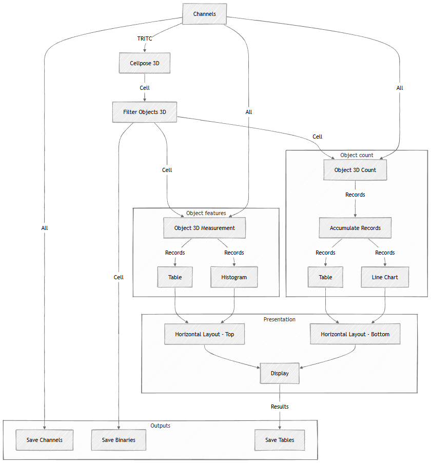
Figure 762. Schematic.
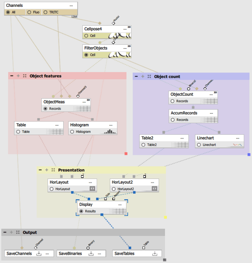
Figure 763. Recipe.
Cellpose 3D segmentation
Cellpose 3D provides AI-powered 3D cell segmentation:
Parameters:
Diameter: 60 pixels - typical cell diameter.
Anisotropy: 2 - cell model type.
Cellpose 3D considers all Z-slices simultaneously, producing accurate 3D cell segmentations.
Note
Anisotropic resolution handling: Because Z-resolution is typically worse than XY, set the Z-scale parameter to account for this. For example, if XY = 0.1 µm/pixel and Z = 0.5 µm/slice, the anisotropy ratio is 5:1. Cellpose uses this to properly weight 3D shape detection.
Filter Objects 3D
Filter Objects 3D removes objects by 3D criteria:
Filtering:
Feature: Equivalent Diameter (3D).
Comparator: Greater than.
Value: 5 µm.
Removes objects smaller than 5 µm equivalent diameter, filtering out debris and segmentation artifacts.
Object 3D Count
Same as Workflow 1: provides per-volume summary statistics including object count, total volume, and mean intensities across volumes.
Object 3D Measurement
Measures comprehensive 3D features for each segmented object:
3D morphology:
Volume, surface area.
Width, height, depth (bounding box).
Sphericity, elongation ratios.
Position (center X, Y, Z).
3D intensity:
Mean, max, min, sum across all channels.
Standard deviation within object.
Each row represents one 3D object.
Accumulate Records
Collects per-volume counts across the time series:
Tracks object count changes.
Accumulates summary statistics.
Visualization
Shows 3D features of all objects in the displayed volume. Selecting rows highlights objects in the 3D viewer.
Displays object counts and aggregated features across all volumes.
Shows distribution of any 3D feature (e.g., volume distribution, sphericity distribution) for current volume. Includes normal fit overlay.
Plots temporal evolution of object count or aggregated features (e.g., mean volume over time).
Organize views for easy comparison between current volume details and time-series trends.
Results
This workflow produces:
3D segmentation masks for all cells/objects.
Comprehensive 3D morphological measurements per object.
Intensity statistics in 3D volumes.
Temporal trends in object count and features.
Feature distributions with statistical fits.
Use cases
Organoid growth tracking, spheroid morphology analysis, 3D cell shape characterization, volumetric tumor analysis.
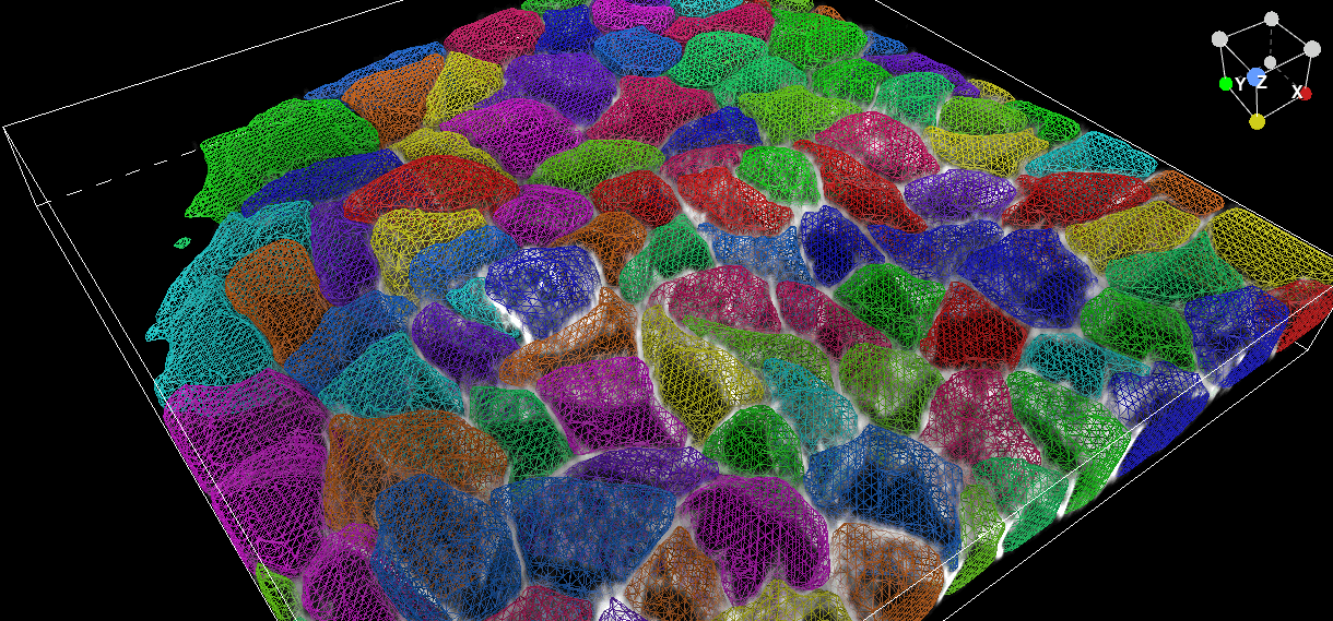
Figure 764.
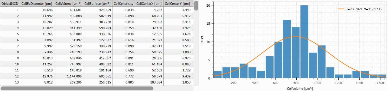
Figure 765.
Table 23. Workflow selection guide.
| Workflow | Segmentation | Analysis type | Output | Best for |
|---|---|---|---|---|
| 3D Object Count | Bright Spots 3D | Population stats | Counts per volume | Simple 3D spot counting |
| 3D Particle Tracking | Bright Spots 3D | Motion analysis | 3D trajectories | Particle movement in 3D |
| 3D Object Measurement | Cellpose 3D | Morphology | Individual features | Complex 3D shape analysis |
Table 24. Parameter comparison.
| Parameter | Object Count | Particle Tracking | Object Measurement |
|---|---|---|---|
| Segmentation | Bright Spots 3D | Bright Spots 3D | Cellpose 3D + Filter |
| Main node | Object 3D Count | Track Particles 3D | Object 3D Measurement |
| Output level | Per-volume | Per-particle | Per-object |
| Temporal analysis | Count trends | 3D trajectories | Morphology trends |
Resolution anisotropy
Problem: Z-resolution typically 3-5× worse than XY resolution, causing:
Distorted object shapes (spheres appear elongated).
Biased measurements (overestimated surface area).
Poor segmentation along Z.
Solutions:
Use isotropic acquisition when possible.
Set proper Z-scale in Cellpose 3D.
Apply resolution-aware measurements.
Resample to isotropic voxels if needed.
Computational demands
3D processing requires significantly more:
Memory: 100× more voxels than single slice.
Processing time: Volume operations are slower.
Storage: Larger file sizes.
Solutions:
Use binning (2×2 or 2×2×2) if resolution permits.
Crop to region of interest in XY and Z.
Process subsets of time points.
Use GPU-accelerated nodes when available.
Z-drift and focus issues
Problem: Focus may drift during acquisition:
Objects move out of focus.
Inconsistent segmentation across volumes.
Tracking failures.
Solutions:
Use hardware autofocus during acquisition.
Apply focus correction before analysis.
Crop Z-range to consistently focused region.
Use perfect focus systems.
Limited Z-coverage
Problem: Objects may exit the imaged volume:
Incomplete 3D structures at top/bottom.
Tracking breaks when particles leave volume.
Biased measurements near boundaries.
Solutions:
Acquire larger Z-range.
Filter border objects in Z dimension.
Account for partial volumes in analysis.
Use Remove Border Objects 3D node.
Acquisition optimization
Z-stack parameters:
Z-step: Follow Nyquist criterion: step ≤ λ/(2·NA·n) for optimal sampling.
Z-range: Cover full object extent plus margin.
Speed: Balance temporal resolution vs. photobleaching.
Focus: Use autofocus or perfect focus system.
Resolution:
Aim for isotropic if possible (same XY and Z resolution).
At minimum: Z ≤ 3× XY spacing.
For sphericity measurements: Z ≤ 2× XY preferred.
Signal quality:
Adequate signal-to-noise ratio throughout Z-stack.
Minimize photobleaching (optimize laser power, dwell time).
Uniform illumination across Z-range.
Segmentation strategies
For sparse objects (particles, spots):
Use Bright Spots 3D with appropriate diameter.
Set contrast threshold conservatively.
Verify detection at multiple Z-positions.
For dense objects (cells, organoids):
Use Cellpose 3D for best results.
Set diameter to typical object size.
Adjust Z-scale for anisotropic resolution.
Filter by size to remove artifacts.
For irregular structures:
Use 3D Threshold with appropriate cleaning.
Apply 3D smoothing before segmentation.
Consider watershed-based separation.
Measurement validation
Visual verification:
Inspect segmentation overlays in image and volume view.
Verify object boundaries at top and bottom of stack.
Check that 3D renderings match expected morphology.
Quality metrics:
Monitor segmentation consistency across volumes.
Validate against manual measurements.
3D deconvolution
For improved resolution and contrast:
Apply before segmentation.
Use appropriate PSF for your system.
Balance deconvolution iterations vs. artifacts.
Surface rendering
For publication-quality visualization:
Use 3D viewer with volume rendering.
Adjust transfer functions for optimal display.
Create rotating animations.
Export high-resolution images.
Multi-channel 3D analysis
Analyze relationships in 3D:
Segment each channel independently.
Calculate 3D colocalization.
Measure inter-object distances in 3D.
Analyze 3D spatial distributions.
4D analysis (3D + time)
For dynamic processes:
Track objects in 3D across time.
Measure morphology changes in 4D.
Analyze 3D cell divisions.
Track organoid growth over days.
Table 25. Memory estimates.
| Image size | Bit depth | Volumes | RAM needed |
|---|---|---|---|
| 512×512×50 | 16-bit | 100 | ~5 GB |
| 1024×1024×100 | 16-bit | 100 | ~40 GB |
| 2048×2048×100 | 16-bit | 50 | ~80 GB |
Processing time estimates
Relative to 2D processing:
3D Spot Detection: 10-20× slower.
Cellpose 3D: 20-50× slower (GPU recommended).
3D Measurements: 5-10× slower.
3D Tracking: 2-5× slower (fewer time points usually).
Optimization strategies
Reduce data size:
Crop to ROI before processing.
Bin 2×2 (reduces to 1/4 data).
Process subset of time points first.
Use GPU acceleration:
Cellpose 3D benefits significantly.
Some measurement nodes support GPU.
Check node documentation.
Batch processing:
Process multiple files overnight.
Use Job Manager for automation.
Parallelize independent analyses.
Poor segmentation
Symptoms: Objects split across slices, fragmented structures, missing objects.
Causes:
Inadequate Z-resolution.
Poor signal-to-noise ratio.
Wrong segmentation parameters.
Solutions:
Improve acquisition (smaller Z-step, better SNR).
Use 3D smoothing before segmentation.
Adjust diameter and contrast settings.
Try Cellpose 3D instead of threshold.
Incorrect measurements
Symptoms: Unrealistic volumes, wrong sphericity, inconsistent values.
Causes:
Incorrect calibration (especially Z).
Anisotropic resolution not accounted for.
Border effects.
Solutions:
Verify XY and Z calibration.
Check metadata in image file.
Set proper Z-scale in analysis nodes.
Remove border objects.
Tracking failures in 3D
Symptoms: Broken tracks, ID swapping, missing particles.
Causes:
MaxSpeed too small for 3D movement.
Particles leaving Z-range.
Segmentation inconsistency.
Solutions:
Increase maxSpeed to account for Z-displacement.
Use maxGap to bridge temporary disappearances.
Improve segmentation consistency.
Crop to central Z-region.
Performance issues
Symptoms: Out of memory errors, excessive processing time.
Causes:
Large 3D datasets.
Insufficient RAM.
Inefficient processing.
Solutions:
Process smaller Z-ranges.
Use binning to reduce data size.
Add more RAM.
Process volumes in batches.