
Time measurement (also called field measurement over time) quantifies how intensity changes throughout a time-lapse sequence. Unlike object counting workflows that detect and count individual objects, time measurement focuses on aggregate intensity within defined regions - either the entire field of view or specific regions of interest (ROIs).
This is one of the simplest yet most powerful workflows in GA3, commonly used to track:
Calcium signaling (fluorescence changes in cells).
Bleaching kinetics (fluorophore photobleaching over time).
Expression dynamics (protein expression levels).
Drug responses (intensity changes after treatment).
Multi-channel comparisons (ratio imaging, FRET).
Both workflow variants produce temporal intensity data but differ in scope and organization:
Channel-based workflow (whole field or single mask):
Table showing mean, max, min intensity per frame across all channels.
Line chart with separate traces for each channel.
Simple comparison of multiple channels in the same region.
ROI-based workflow (multiple regions):
Table pivoted to show each ROI as a separate column.
Line chart with one trace per ROI (color-coded).
Comparison of intensity dynamics across multiple spatial regions.
Both produce synchronized displays where clicking a table row jumps to the corresponding time point in the image.
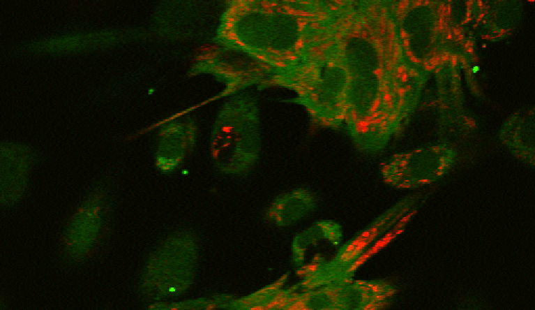
Figure 699.
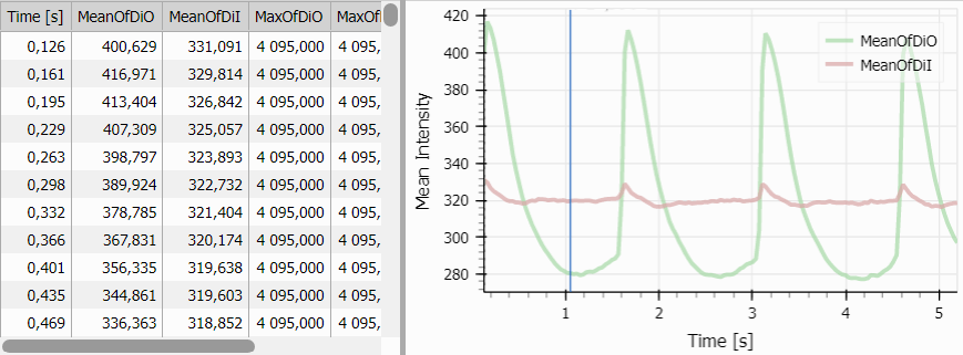
Figure 700.
Workflow overview
Time measurement workflows consist of four core components:
Define measurement region(s)
Either use the entire field, draw a single mask, or draw multiple ROIs.
Measure intensity features
Extract mean, max, min intensity values per frame.
Accumulate over time
Collect measurements from all frames into a single table.
Visualize temporal trends
Display data as tables and line charts showing intensity evolution.
This workflow comes in two main variants that share similar structure but differ in how they define and process measurement regions:
Variant 1: Channel-based (whole field or single mask)
Use case: Compare intensity changes across multiple channels in the same region.
Key features:
Optional single ROI/mask applied globally.
Measures all channels simultaneously.
One row per frame with columns for each channel and statistic.
Line chart displays multiple channels as separate series.
When to use:
Comparing channel dynamics (e.g., FRET ratio imaging).
Tracking overall field intensity.
Measuring intensity in one defined region across channels.
Variant 2: ROI-based (multiple regions)
Use case: Compare intensity dynamics across multiple spatial locations in a single channel.
Key features:
User draws multiple ROIs (2-20+ regions).
Measures selected channel in each ROI.
Cross-tabulated view with ROIs as columns.
Line chart displays one trace per ROI.
When to use:
Comparing different cells or cellular compartments.
Tracking independent regions simultaneously.
Measuring local vs. global responses.
Ratio measurements between specific locations.
Note
The key difference: Channel workflow measures multiple channels in one region; ROI workflow measures one channel in multiple regions. Choose based on whether you are comparing channels or comparing locations.
This simpler variant measures intensity across all channels in a single field or masked region.
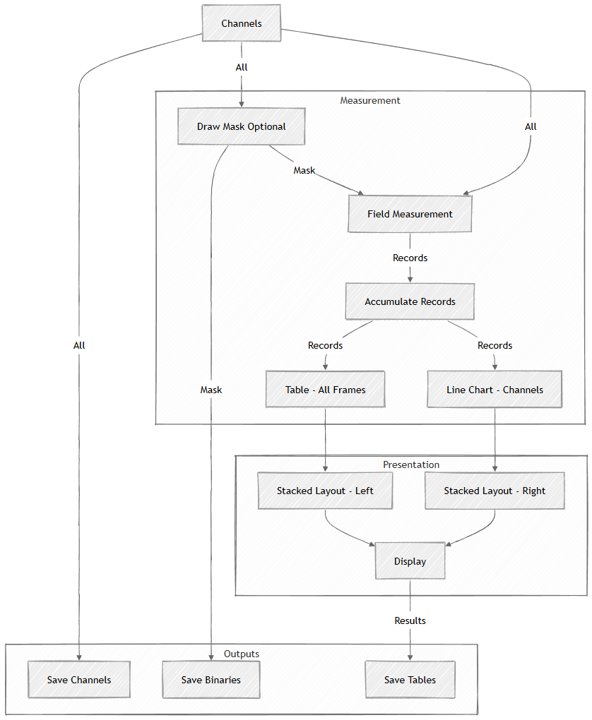
Figure 701. Schematic.
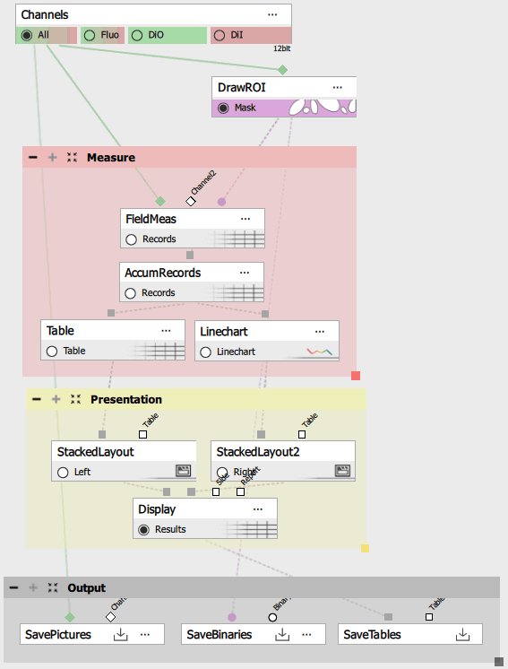
Figure 702. Recipe.
Drawing the measurement mask (optional)
To draw a ROI/Mask use Segmentation > Interactive > Draw Objects. That allows defining a region of interest interactively when the recipe runs.
Key features:
Interactive drawing: When the recipe executes, a dialog appears prompting you to draw a region.
Drawing tools: Rectangle, ellipse, polygon, freehand.
Optional: If no mask is drawn, the entire field is measured.
Persistent: Once drawn, the same mask applies to all frames in the time-lapse.
How it works:
Run the recipe.
Drawing dialog appears overlaid on the image.
Select a drawing tool and define the region.
Click OK to proceed with measurement.
The mask output is a binary layer that restricts the measurement to pixels inside the drawn region.
Note
When to use a mask:
Focus on a specific cell or region.
Exclude background or edge artifacts.
Measure intensity in a defined cellular compartment.
Compare intensity inside vs outside a region (requires two separate measurements).
When to skip the mask:
Measuring the entire field.
Uniform sample with minimal background.
Comparing overall intensity across channels.
Field Measurement
Measurement > Basic > Field computes intensity statistics for the entire field or masked region. This is a field-level measurement, meaning it produces one value per frame (not per object).
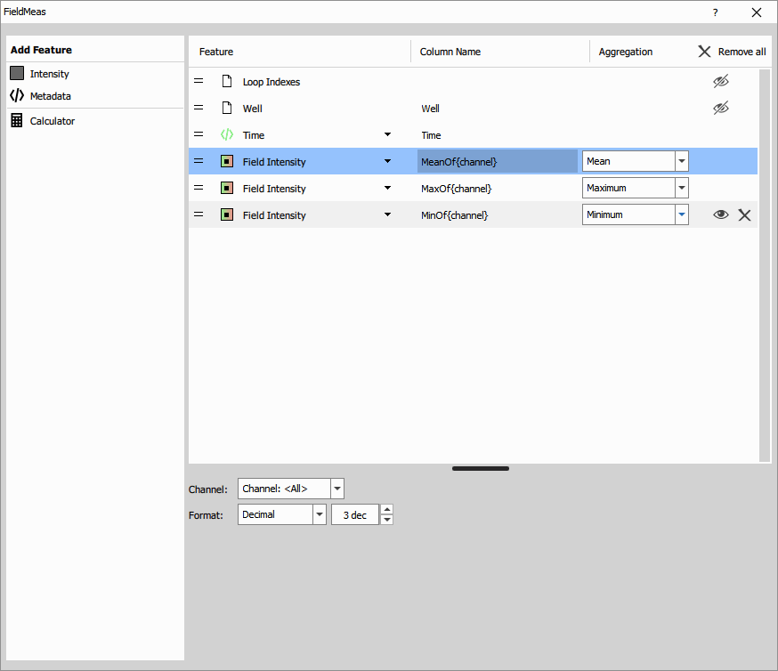
Figure 703.
Inputs:
Channel(s): The intensity channels to measure.
Mask: Binary layer restricting the measurement region.
Measured features:
System features (automatic):
Loop Indexes: Frame number.
WellName: Well identifier (for multi-well plates).
Time: Timestamp in seconds.
Intensity features (per channel):
Mean Intensity: Average pixel intensity in the region.
Maximum Intensity: Brightest pixel value.
Minimum Intensity: Dimmest pixel value.
Aggregation: Each intensity feature is measured per channel. With 3 channels, you get:
MeanIntensity (DAPI).
MeanIntensity (FITC).
MeanIntensity (Texas Red).
MaximumIntensity (DAPI).
MaximumIntensity (FITC).
etc.
The node produces one row per frame, with columns for all measured features across all channels.
Note
Mask behavior: If a mask is connected to the Interactive drawing it can handle empty mask and ignores it (as if it was not connected). Otherwise an empty mask produces no measurement.
Accumulate Records
Data manipulation > Basic > Accumulate Records collects measurements from all frames into a single table.
Settings:
LoopName: “All loops” (accumulate over all loops - time, z-stack, multi-point).
Without accumulation, only the current frame’s measurement would be available. Accumulation enables temporal analysis of the entire time-lapse.
Results Table
Table displays the accumulated intensity measurements.
Configuration:
Data/Display: “All data” to show all frames.
Interaction/Row selection: Enabled for frame navigation.
Statistics: Min, max, mean of each column.
Table 15. Table structure (example with 2 channels).
| Time [s] | MeanIntensity (DAPI) | MeanIntensity (FITC) | MaxIntensity (DAPI) | MaxIntensity (FITC) |
|---|---|---|---|---|
| 0.000 | 1245.3 | 876.2 | 4095 | 3821 |
| 2.156 | 1198.7 | 823.1 | 4012 | 3654 |
| 4.312 | 1156.4 | 779.8 | 3945 | 3498 |
Interactive features:
Click a row to navigate to that time point.
Sort by any column to find max/min values.
Statistics panel shows overall trends.
Line Chart
Results & Graphs > Graphs > Linechart visualizes intensity changes over time.
Configuration:
X-axis: Time (formatted as time).
Y-axis: All intensity features (mean, max, min).
Color coding: Automatic channel-based palette.
Display: “All data” to plot entire time series.
Chart features:
Multiple traces: Each channel’s intensity plotted separately.
Color-coded: Matches the channel colors from the image.
Interactive tools: Pan, zoom, frame selection.
Legend: Shows/hides individual traces.
The chart immediately reveals:
Photobleaching (declining intensity).
Calcium transients (sharp intensity spikes).
Baseline stability.
Channel relationships (increasing/decreasing together).
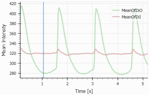
Figure 704.
Layout and Display
Two Stacked Layout nodes (Results & Graphs > Layout > Stacked) organize the views:
Left pane: Results table.
Right pane: Line chart.
Results & Graphs > Layout > Display combines these with the image viewer into a synchronized interface:
Selecting a table row jumps to that frame.
The current frame is highlighted in the table.
Chart shows temporal position of current frame.
This variant measures intensity in multiple user-defined regions, useful for comparing dynamics across different spatial locations.
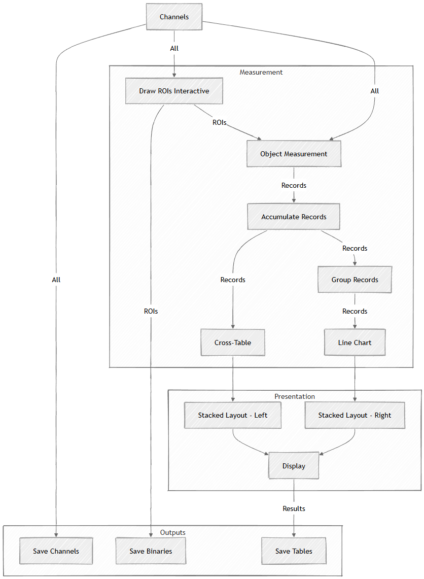
Figure 705. Schematic.

Figure 706. Recipe.
Drawing Multiple ROIs
To draw ROIs use Segmentation > Interactive > Draw Objects. It enables drawing multiple regions of interest that are treated as separate objects.
Key differences from single mask:
Multiple regions: Draw 2-20+ separate ROIs.
Each ROI = object: Each region gets a unique Object ID.
Independent measurement: Each ROI measured separately.
Persistent across frames: All ROIs apply to every frame in the time-lapse.
Interactive drawing workflow:
Run the recipe.
Drawing dialog appears.
Draw first ROI (rectangle, polygon, etc.).
Click “Add” to create additional ROIs.
Each new region becomes a separate object.
ROIs are numbered automatically (ROI 1, ROI 2, etc.).
Click OK when all regions are defined.
ROI organization:
ROIs are stored as a binary layer with object IDs.
Each pixel has a value: 0 (background), 1 (ROI 1), 2 (ROI 2), etc.
ROIs can overlap (last-drawn takes precedence).
ROIs can be any shape (circles, polygons, freehand).
Note
ROI placement strategies:
Cell comparison: Draw one ROI per cell to compare individual cell responses.
Compartment analysis: Draw ROIs on nucleus, cytoplasm, membrane.
Spatial gradients: Draw ROIs across the field to detect spatial patterns.
Reference regions: Include background ROI for normalization.
Object Measurement on ROIs
Object/ROI Measurement (Measurement > Basic > Object) treats each ROI as an object and measures intensity features within it.
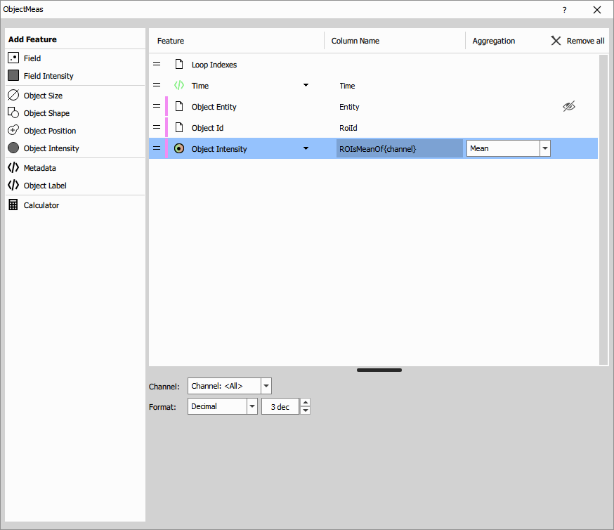
Figure 707.
Inputs:
Binary (ROIs): The drawn ROIs as separate objects.
Channel: The intensity channel to measure.
Important difference from field measurement:
Field measurement → one row per frame.
Object measurement → one row per ROI per frame.
With 2 ROIs and 100 frames, this produces 200 rows (2 ROIs × 100 frames).
Measured features:
System features:
ObjectId: ROI identifier (1, 2, 3, etc.).
Time: Timestamp for this frame.
Intensity features (per ROI, per frame):
Mean Intensity: Average intensity in this ROI.
Additional features: Max, min, sum, standard deviation (configurable).
The key insight: Each ROI is measured independently at every time point, enabling direct comparison of temporal dynamics across regions.
Accumulate Records
Data manipulation > Basic > Accumulate Records collects all ROI measurements across all frames.
Settings:
LoopName: “All loops” (accumulate over time).
The accumulated table contains all ROIs in all frames:
This “long format” table has ROI and time on separate axes, requiring reshaping for easy comparison.
Group Records by ROI
Data manipulation > Grouping > Group Records organizes the data by ROI for visualization.
Settings:
Selected Columns: ObjectId (grouped by ROI).
Purpose: Prepares the data for line chart plotting where each ROI should be a separate trace. Grouping creates a hierarchical structure:
Group 1 (ROI 1): All time points for ROI 1.
Group 2 (ROI 2): All time points for ROI 2.
etc.
This allows the line chart to automatically create one trace per ROI with appropriate colors.
Cross-Tab (Pivoted Table)
Results & Graphs > Tables > Cross Table reshapes the table to show ROIs as columns instead of rows.
Configuration:
Data/Display: “All data”.
Pivot Enabled: Yes.
Pivot Column: ObjectId (ROI).
Pivot Direction: “Grouped” (one column per ROI value).
Table transformation:
Before (long format):
After (pivoted format):
Benefits:
One row per time point (easier to read).
Direct comparison across ROIs.
Suitable for exporting to spreadsheet software.
Each ROI is a separate column.
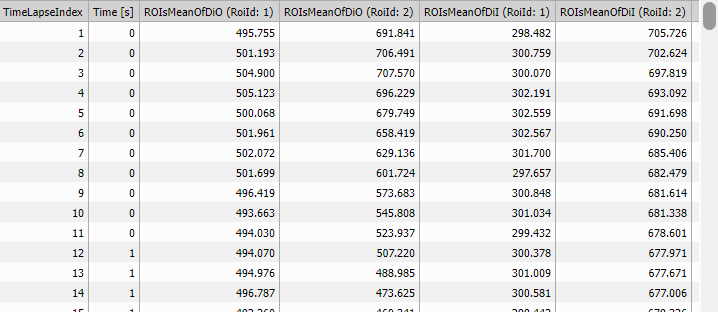
Figure 708.
Line Chart (ROI traces)
Results & Graphs > Graphs > Linechart displays one trace per ROI.
Configuration:
X-axis: Time (formatted as time).
Y-axis: Mean Intensity (from grouped data)
Grouping: By ObjectId (one trace per ROI)
Color palette: “Object” palette (assigns distinct colors).
Chart features:
Multiple traces: Each ROI plotted as a separate colored line.
Color-coded legend: Shows which color corresponds to which ROI.
Synchronized: Clicking the chart navigates to that time point.
Interactive tools: Pan, zoom, select frames.
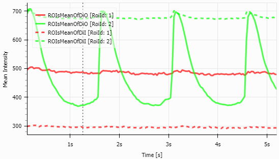
Figure 709.
This visualization immediately shows:
Which ROIs respond similarly (parallel traces).
Which ROIs have different dynamics (diverging traces).
Temporal relationships (which ROI peaks first).
Amplitude differences (which ROI has strongest signal).
Layout and Display
Two Stacked Layout nodes (Results & Graphs > Layout > Stacked) organize:
Left pane: Cross-tabulated table (ROIs as columns).
Right pane: Line chart (one trace per ROI).
Results & Graphs > Layout > Display creates a synchronized interface:
Selecting a table row jumps to that time point.
Clicking on the chart navigates the image.
ROI selection in image highlights corresponding table column.
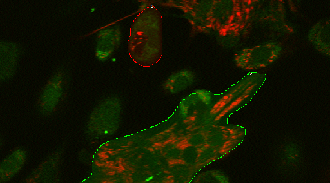
Figure 710.
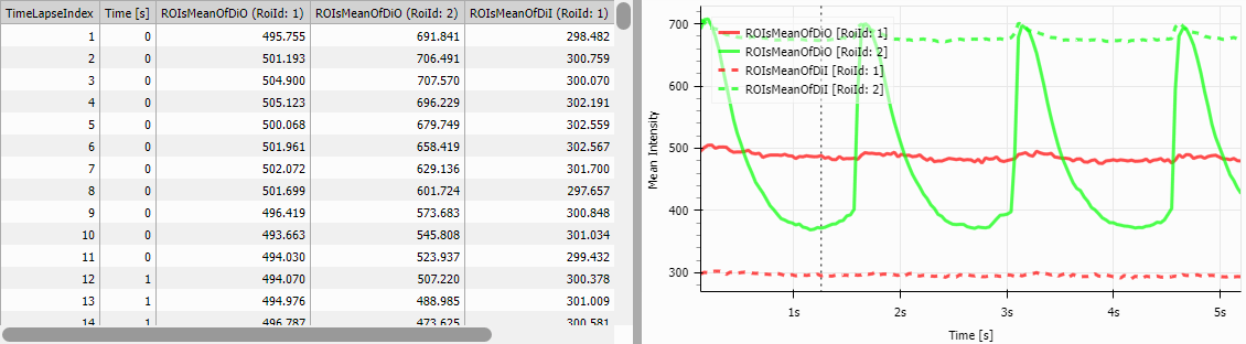
Figure 711.
When to use Channel-based workflow
Best for:
Multi-channel imaging with co-localized signals.
Ratio imaging (e.g., FRET, ratiometric calcium indicators).
Comparing different fluorophores in the same region.
Simple whole-field intensity tracking.
Advantages:
Simpler workflow (fewer nodes).
Automatic channel handling.
Single-region focus reduces complexity.
Easier to set up.
Limitations:
Only one measurement region (or full field).
Cannot compare different spatial locations.
Less suitable for heterogeneous samples.
When to use ROI-based workflow
Best for:
Comparing multiple cells or regions.
Subcellular compartment analysis (nucleus vs. cytoplasm).
Spatial heterogeneity studies.
Single-cell time traces within a population.
Local vs. global response comparison.
Advantages:
Multiple independent measurements.
Spatial comparison capability.
Flexible ROI placement.
Each ROI tracked separately.
Limitations:
Requires interactive ROI drawing.
More complex data structure (requires pivoting).
Limited to one channel per workflow (run multiple times for multi-channel).
Table 19. Parameter comparison
| Feature | Channel-based | ROI-based |
|---|---|---|
| Measurement node | Field Measurement | Object Measurement |
| Regions | 0-1 (full field or mask) | 2-20+ (multiple ROIs) |
| Channels | All channels measured | Single channel |
| Table format | One row per frame | Pivoted (ROIs as columns) |
| Chart | One trace per channel | One trace per ROI |
| Complexity | Simple | Moderate |
Background subtraction
Measure a background ROI and subtract from other ROIs:
Include one ROI in a background region.
After accumulation, use Data manipulation > JavaScript > JS Create Column.
Calculate: CorrectedIntensity = MeanIntensity - BackgroundIntensity.
Ratio measurements
Create ratiometric traces (e.g., FRET ratio):
Run channel-based workflow measuring donor and acceptor channels.
Calculate: Ratio = MeanIntensity(Acceptor) / MeanIntensity(Donor)
Plot ratio over time.
Normalized intensity
Normalize to baseline or peak:
After accumulation, use Reduce Records.
Calculate baseline mean (first 10 frames).
Use Create Column: NormalizedIntensity = (Intensity - Baseline) / Baseline
Express as ΔF/F0 (fractional change).
Multi-channel ROI analysis
Measure multiple channels in the same ROIs:
Run the ROI workflow once per channel.
Save each result separately.
Use Join Records (
 Data manipulation) to merge tables.
Compare channel dynamics in each ROI.
ROI drawing strategy
For single cells:
Draw ROIs tightly around cell boundaries.
Avoid including intercellular space.
Use ellipse or polygon tools for accurate fit.
Number ROIs consistently if comparing across experiments.
For subcellular compartments:
Draw nuclear ROI first (usually brightest).
Draw cytoplasmic ROI excluding nucleus.
Include background ROI for normalization.
Ensure ROIs do not overlap (or manage overlap intentionally).
For field gradients:
Draw ROIs in a grid pattern.
Use consistent ROI sizes.
Number ROIs in spatial order (left to right, top to bottom).
Choosing measurement statistics
Mean intensity:
Most commonly used.
Robust to small spatial variations.
Represents average signal level.
Maximum intensity:
Useful for detecting peaks (calcium spikes).
Sensitive to noise.
Good for sparse signals.
Minimum intensity:
Estimates baseline level.
Useful in bleaching studies.
Less commonly used.
Sum intensity:
Total signal in the ROI.
Depends on ROI size.
Useful when ROI size matters (growing/shrinking regions).
Temporal analysis strategies
For photobleaching correction:
Fit exponential decay to intensity data.
Calculate bleaching time constant.
Normalize later time points using fitted curve.
For response quantification:
Define baseline period (before stimulus).
Calculate baseline mean and standard deviation.
Define response threshold (e.g., baseline + 3×SD).
Measure response amplitude and duration above threshold.
Performance optimization
For long time-lapses:
Use “Apply only on current frame in preview” in Accumulate Records.
Process a subset of frames first to verify settings.
Consider downsampling time points (every Nth frame) if temporal resolution allows.
For many ROIs:
Limit to essential ROIs (10-20 max).
Use rectangular ROIs when possible (faster computation).
Consider batch processing if analyzing multiple datasets.
No data in table / empty results
Cause: Mask or ROI not drawn, measurement fails.
Solution:
Check that ROIs are actually drawn (should see colored overlays).
For channel-based: disconnect mask input if not using a mask.
Line chart shows all ROIs as one trace
Cause: Group Records not applied correctly.
Solution:
Verify Group Records is connected between Accumulate and Line Chart.
Check that grouping is by ObjectId.
Line chart palette should be set to “object” or “group”.
Intensity values seem wrong
Cause: ROI placement, channel selection, or bit depth issues.
Solution:
Verify ROIs are in the correct regions (not in background).
Check that correct channel is connected to measurement.
Compare with image histogram.
Cross-tab not showing ROIs as columns
Cause: Pivot settings incorrect.
Solution:
Ensure Pivot Enabled is checked.
Pivot Column should be ObjectId (or _ObjId)
Pivot Direction should be “grouped” or “wide”.
Chart time axis not formatted correctly
Cause: Axis format not set to “time”.
Solution:
In Line Chart settings, set X-axis labels_format to “time”.
Verify Time column is selected for X-axis.
Add curve fitting
After accumulation, use Fit node ( Data manipulation) to:
Fit exponential decay for bleaching analysis.
Fit sigmoidal curve for dose-response.
Extract kinetic parameters.
Add statistical analysis
Use statistical nodes to:
Calculate mean and SEM across replicates.
Compare baseline vs. stimulated periods with t-tests.
Quantify response amplitude and latency.
Add automated ROI detection
Replace Draw ROIs with segmentation:
Use Threshold or Segmentation > Special detections > Cellpose4 to detect cells automatically.
Each detected object becomes an automatic ROI.
Useful for large-scale analysis.
Add time-course normalization
Use Data manipulation > JavaScript > JS Create Column to:
Normalize to initial frame (t=0).
Express as percentage of maximum.
Calculate z-scores.
Both workflows save:
Save Channels
Input & Output > Save to Document > Save Channels does not modify channel data as it “stores” the source (Original):
All input channels (RGB or fluorescence).
Original intensity values preserved.
Save Binaries
Input & Output > Save to Document > Save Binaries saves the segmentation results:
Drawn mask (channel-based workflow).
Drawn ROIs (ROI-based workflow).
Save Tables
Input & Output > Save to Document > Save Tables saves all measurement results:
Data is saved into H5 file.
Time-series intensity table.
Can be exported to Excel/CSV.
Includes all measured features.
Time measurement is a versatile workflow for quantifying intensity changes throughout time-lapse sequences:
Best for multi-channel comparisons in single regions. Simple setup, automatic channel handling, ideal for ratio imaging and whole-field tracking.
Best for spatial comparisons within single channels. More complex but powerful for comparing multiple cells, compartments, or regions independently.
Both variants produce synchronized displays linking temporal data to images, enabling exploration of intensity dynamics. Choose the variant that matches your experimental question: comparing channels or comparing locations.