
Shows how to detect nuclei and then use them to detect cells. Nuclei are usually easier to detect due to their contrast and round shape. Here cells are detected by growing nuclei until they fill whole space or the intensity reaches background levels.
This workflow produces:
Well-formed cells (each with exactly one nucleus and non-empty cytoplasm).
Table with comprehensive cell features including morphology and intensity measurements.
Scatter plot for multivariate feature visualization.
Saved channel images, binary masks, and measurement tables.
Synchronized display linking measurements to visual data.
The result should look like this:
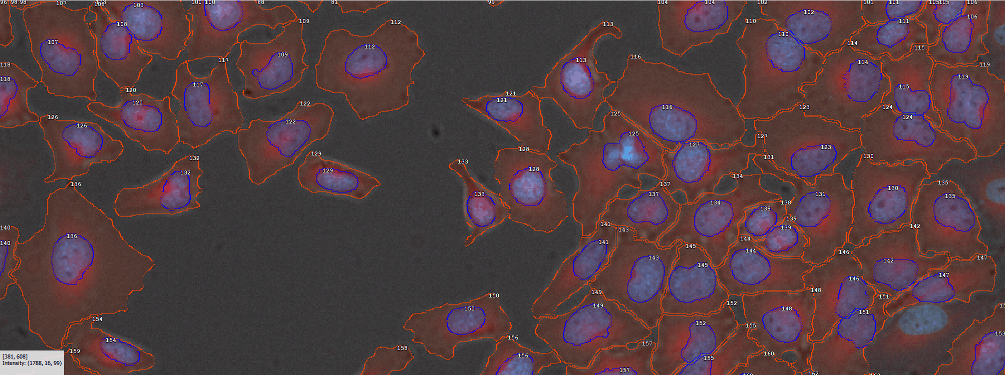
Figure 712.
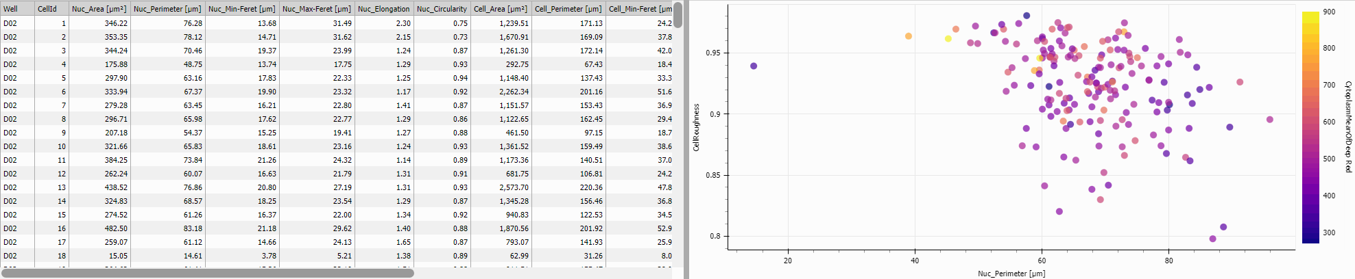
Figure 713.
The recipe consists of:
Nucleus segmentation,
Cell formation block,
Cell measurement and
Presentation block.
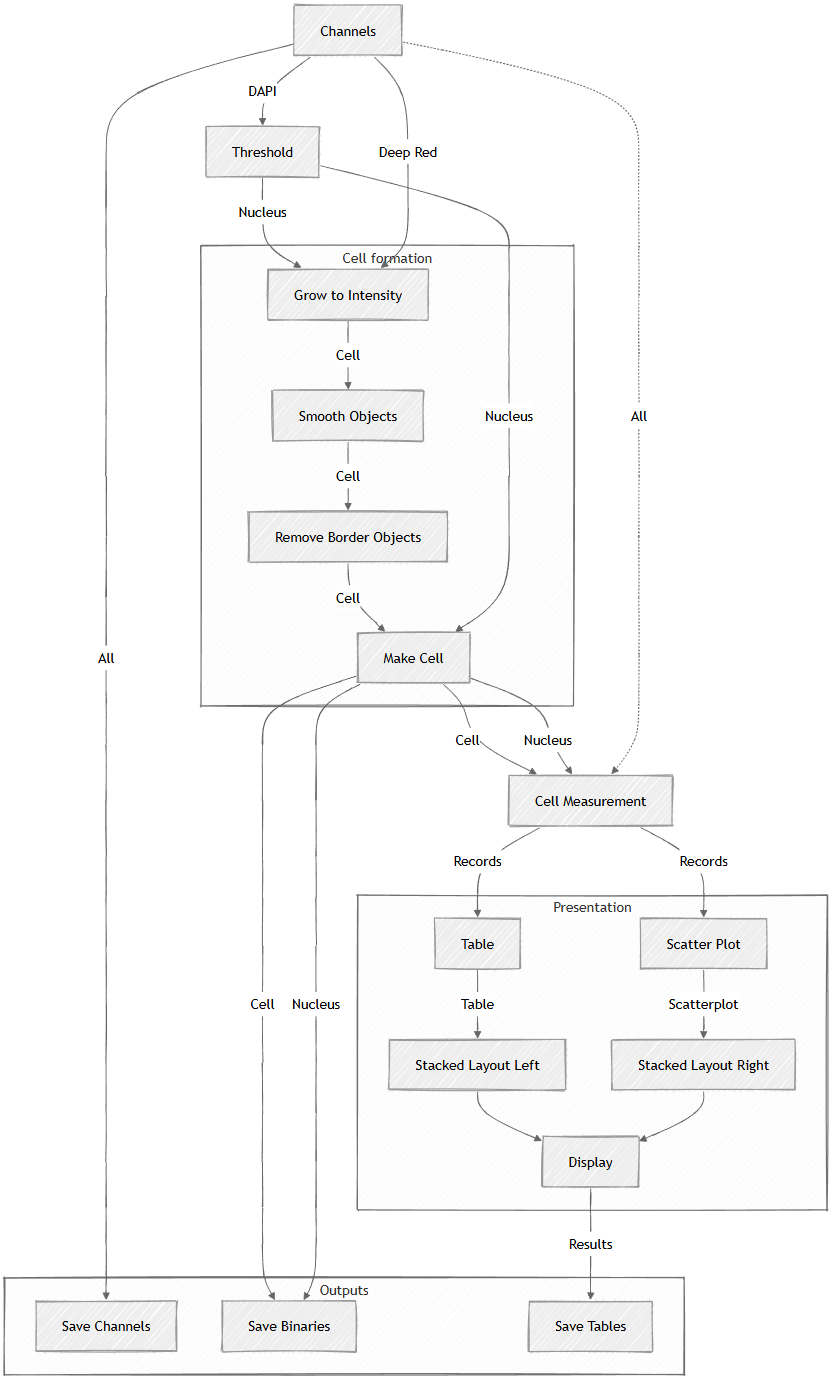
Figure 714. Schematic.
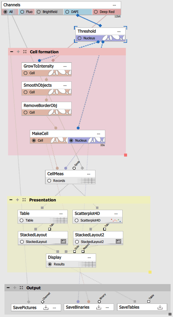
Figure 715. Recipe.
Nucleus detection
Threshold on the DAPI channel creates the initial nucleus segmentation. The nuclear channel is typically the easiest to segment due to:
High contrast between nuclei and background.
Relatively uniform shape and size.
Strong fluorescence signal.
The node uses:
Auto Threshold Method: Triangle algorithm for automatic threshold determination.
Clean: 1.26 µm to remove small artifacts.
Separate: 0.315 µm to split touching nuclei.
Smooth: 0.63 µm to regularize nucleus boundaries.
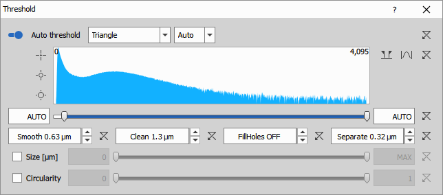
Figure 716.
The cell formation process takes the detected nuclei and grows them to form complete cell boundaries.
Grow to Intensity
Binary processing > Growing > Grow to Intensity expands each nucleus using a watershed algorithm, guided by the intensity of the Deep Red channel. The growth continues until:
The intensity drops below the threshold (ValLow: 150), indicating background.
Another cell is encountered.
The image border is reached.
This technique ensures that each cell has approximately the correct shape and that cells do not overlap.
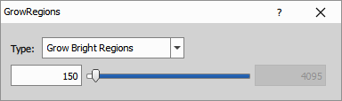
Figure 717.
Smooth Objects
Binary processing > Basic > Smooth Objects with a 2-pixel radius cleans up the cell boundaries, removing small irregularities that can arise from the watershed process.
Remove Border Objects
Binary processing > Remove objects > Touching Borders removes any cells that touch the image border. These cells are typically incomplete and would skew the measurements.
Note
Removing border objects is important for accurate population statistics, as partial cells would artificially lower average cell size and other measurements.
Make Cell
Binary processing > Cell Processing > Make Cell is the critical step that ensures data quality. It validates that each cell is “well-formed” by checking:
Each cell has exactly one nucleus.
Each cell has non-empty cytoplasm (the cell area minus nucleus area).
The area ratio between cell and nucleus is reasonable (< 1000).
Cells that do not meet these criteria are discarded. This node outputs two binary layers:
Cell (R1): The validated cell boundaries.
Nucleus (R2): The corresponding nuclei for these cells.
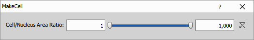
Figure 718.
Measurement > Basic > Cell measures comprehensive features for each validated cell. The node takes three inputs:
Cell binary: Defines the cell boundaries.
Nucleus binary: Defines the nuclear region.
Channel(s): Intensity channels for measurements (optional).
The measurement produces a table with features including:
Morphological features:
Cell area, perimeter, width, height.
Cell circularity and elongation.
Nucleus area, perimeter, width, height.
Nucleus circularity and elongation.
Cytoplasm area (cell area - nucleus area).
Nucleus-to-cell ratio.
Intensity features (when channels provided):
Mean, min, max, standard deviation of intensity.
Per-channel measurements for all input channels.
Each row in the results table represents one cell with all its measured features.
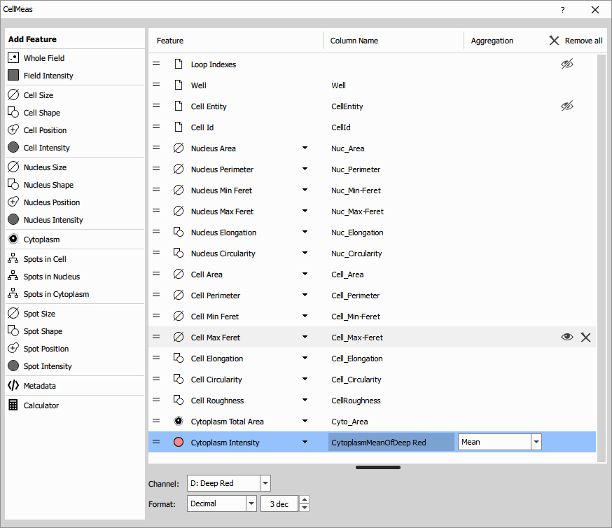
Figure 719.
The presentation block organizes the measurement results into an interactive display with synchronized views.
Table
Table displays the cell measurements with:
Display: Current frame data (frame-by-frame view).
Data Selection: Enabled to allow row selection.
Column Sorting: Enabled for sorting by any feature.
Statistics: Min, max, mean calculations available.
Selecting a row in the table highlights the corresponding cell in the image.
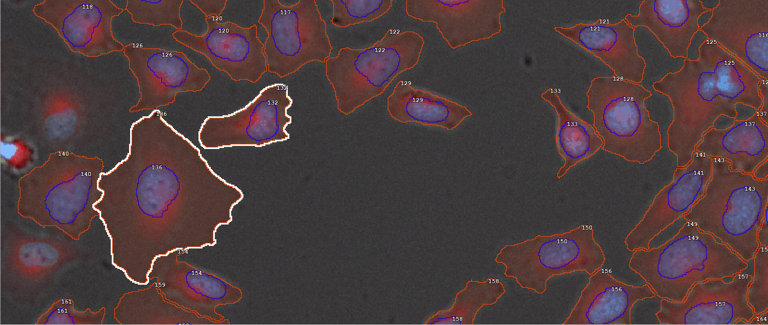
Figure 720.

Figure 721.
Scatter Plot
Results & Graphs > Graphs > Scatterplot 4D provides multivariate visualization with:
X-axis: Configurable feature (e.g., cell area).
Y-axis: Configurable feature (e.g., mean intensity).
Color: Configurable feature (e.g., nucleus-to-cell ratio).
Interactive selection: Click points to select cells in the image.
The scatter plot helps identify cell populations, outliers, and relationships between features.
Use Lasso or rectangle tool to select cluster of similar cells.
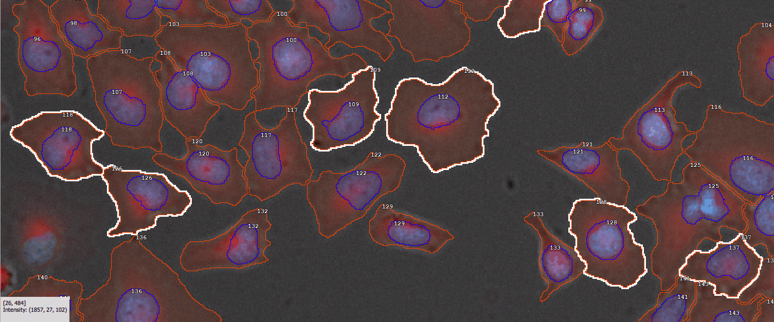
Figure 722.
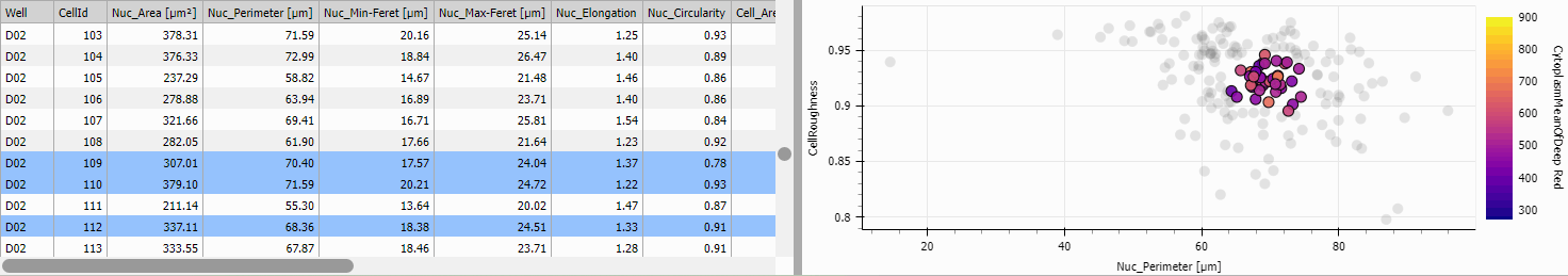
Figure 723.
Layout
Two Stacked Layout nodes (Results & Graphs > Layout > Stacked) organize the visualization:
Left pane: Table showing all cell measurements.
Right pane: Scatter plot for feature correlation analysis.
The Results & Graphs > Layout > Display node combines these layouts into a synchronized interface where:
Selecting cells in the image highlights them in the table and scatter plot.
Selecting rows in the table or points in the scatter plot highlights cells in the image.
All views update together for seamless exploration.
The recipe saves three types of output:
Save Channels
Input & Output > Save to Document > Save Channels saves the original image channels for reference and further analysis.
Save Binaries
Input & Output > Save to Document > Save Binaries saves both:
Cell binary layer: The final validated cell segmentations.
Nucleus binary layer: The corresponding nuclear segmentations.
These can be reloaded later or used for visual verification of segmentation quality.
Save Tables
Input & Output > Save to Document > Save Tables saves the complete measurement table with all cell features.