
(requires: Calcium, FRET)
This “how to” expects you to perform a ratio experiment.
See also: [Ca 2+] Ion Concentration Measurement.
The intended procedure consists of the following portions:
Setting up Optical Configurations
6D: Time and MultiChannel Set Up
Create/ Save/ Open ROIs
Time Measurements Set Up
Capturing data set
Calcium Calibration
Export to Excel/ Text File
Create two optical configurations containing filter settings (use the  Calibration > New Optical Configuration
  command). Call them “340” and “380” (indicating excitation wavelengths).
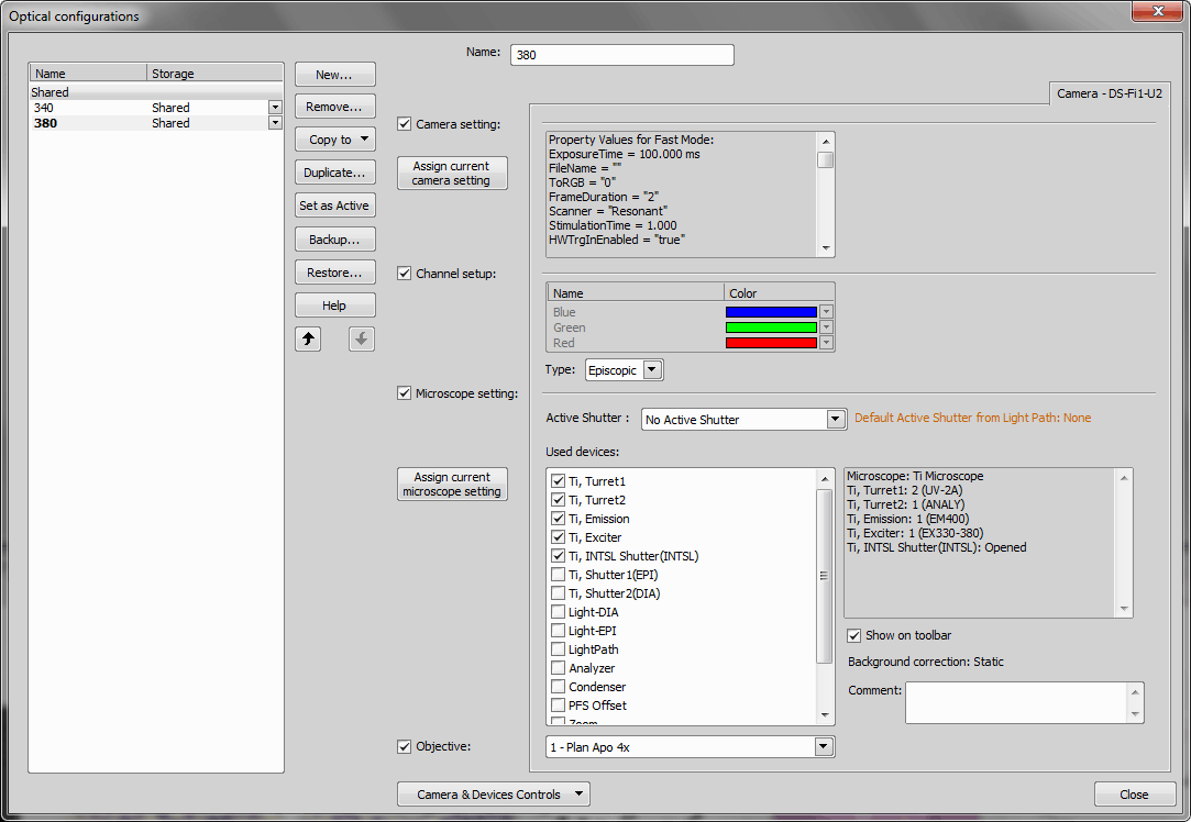
Figure 641.
Note
If different camera settings (exposure, EM gain, etc) are desired for individual channels, then create microscope + camera settings optical configurations.
Active Shutter will most likely be the EPI Shutter.
The only difference between these two Optical Configurations may be the filter state of the excitation of 340 and excitation of 380.
Run the Applications > 6D > Define/Run ND Acquisition  command.
In the Time tab, adjust the settings according to the image:
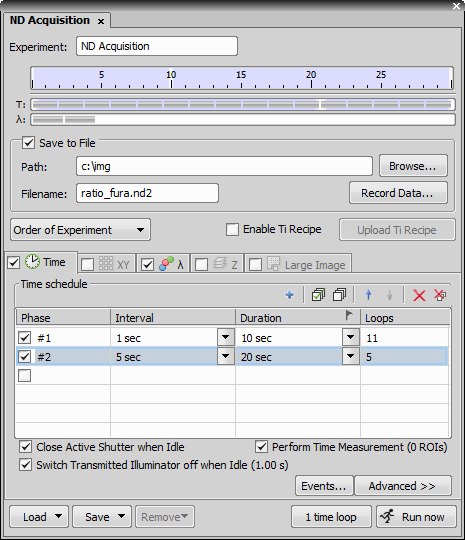
Figure 642.
In the Lambda (wavelength) tab, define two channels:
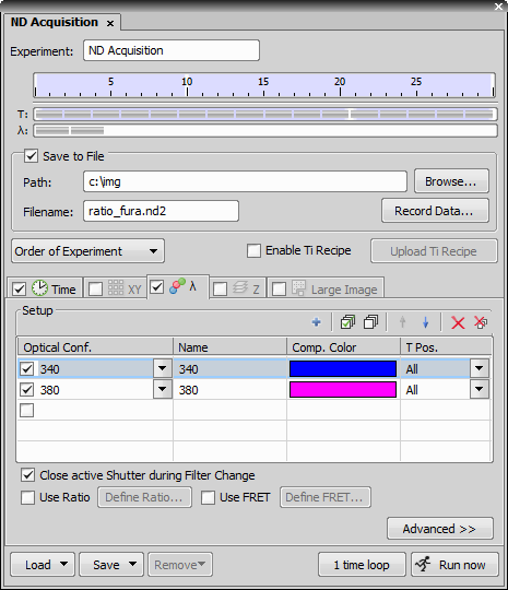
Figure 643.
In the case of 340 and 380, this is a dual excitation experiment. These two channels will share the same emission (510nm). In this case, the component color (pseudocolor) of each of these channels will be the same because NIS-Elements uses the emission wavelength as the default to set the component color. If it is desired to have differing component colors for 340 and 380, then select the drop down list of component colors to change (or both) of the lambdas.
Note
At this point, it is recommended (if not completed already) to optimize the correct camera exposures for 340 and 380. In a typical Fura-2 experiment, 380 emission will appear dimmer than 340, an indicator that cellular calcium is bound, not free. When establishing optimal exposure, be cognizant that in an experiment that induces a release of calcium, the emission of 380 will increase. Set exposures to match the dynamic range of the camera and also the full length of the time-lapse and possible biological responses to drug additions.
In the Time tab, select Use Ratio and press the button.
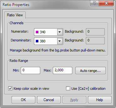
Figure 644.
The Ratio Range is a parameter that specifies the Intensity Modulation Display (IMD). Using the option will automatically scale the IMD based on ratios in the dataset. (Auto range may not be available at the onset of an experiment/ Timelapse because the data for the ratio has not yet been generated.)
Confirm that Perform Time Measurement is checked within the Time tab.
Open up Time Measurement dialog by the
View > Analysis Controls > Time Measurement  command.
Press the button in the 6D dialog window.
Draw several ROIs and one designated to indicate background.
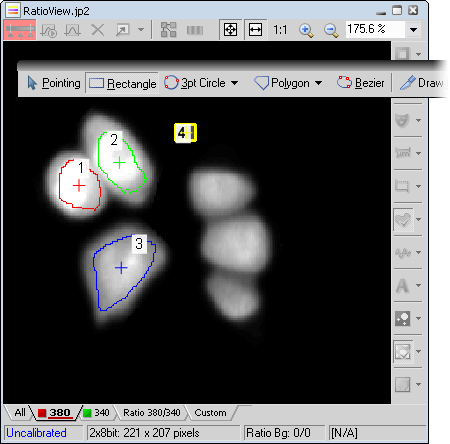
Figure 645.
Right-click the background ROI (#4) and select Use as Background ROI from the context menu.
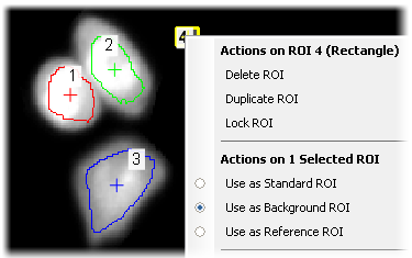
Figure 646.
Once a background ROI is specified, it immediately begins to perform a subtraction and it will be noticeable in the IMD display. The background probe icon
 on the image window will also become active. This drop-down menu provides more options for how to utilize this background ROI. In this case, “Keep Updating Background Offset” is selected.
Save ROIs to a file to be able to load it later. Right-click the ROI button
 on the right image toolbar and select Save ROI As. The ROIs will be saved in a common image format (TIFF, BMP, PNG).
Open up Time Measurement dialog by the
View > Analysis Controls > Time Measurement command (if it has not been already open).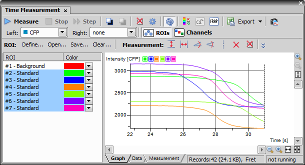
Figure 647.
Highlight (select) all ROIs in order to be displayed in the graph.
At this point in the experiment set up, notice what will be graphed during the Timelapse. Define Left and Right axes display.
Select the display mode - ROIs mode vs. Channels mode. Graphing
 ROIs will graph each cell/ROI individually over time. Graphing
  Channels will graph the average intensity/ ratio of each cell/ ROI over time.
Note
These are graphing options for the during of the Timelapse, but can be modified after acquisition. Choices made at this point in the experimental set up do not affect the data values or limit graph choices post acquisition.
In the 6D dialog window, press the Run Now button. A new image will be captured.
You will be able to observe ratio graphs during the acquisition. This is critical to understand if there is a change in response to the solutions added to the specimen to create ratio responses - a change in the ratio of bound and free calcium in the cells. The live graph is an indication of whether or not there was a response (e.g. if the dose was toxic). This is basically a tool to allow the researcher how to plan the course of the experiment.
Once the full dataset has been measured through the time measurements dialog, it is now possible to set the calcium calibration- normalizing the data off of the experimental Rmin and Rmax.
Select the
 icon.
icon.Pick Rmin value from graph - This is also the Fmax (maximum fluorescence intensity of 380. (Generally speaking this is after EGTA is added and near the start of the calibration routine of the ratio experiment before ionomycin is added).
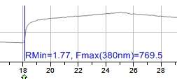
Figure 648.
Pick Rmax value from graph - This is also the Fmin (minimum fluorescence intensity of 380. (Generally speaking this is after ionomycin is added- highest levels of free calcium).
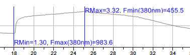
Figure 649.
Click .
What becomes available after calcium calibration
See Exporting Results.