Creating a new recipe

1. Click on Create New in the GPA Explorer, name your new recipe and optionally add some notes, then click OK.

2. GPA Definition window opens. The four main tabs (described below) guide you through the recipe definition.

   

   Figure 270. GPA Definition dialog window.

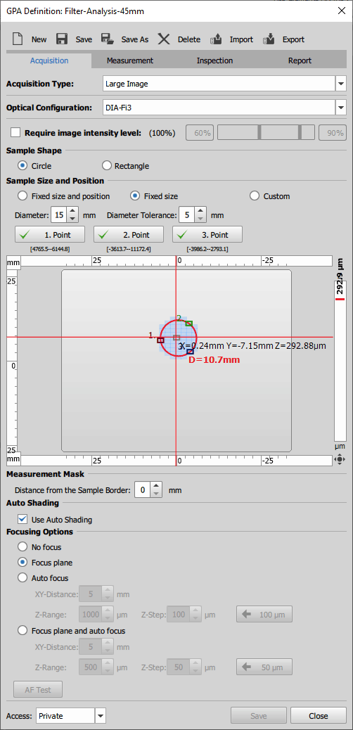
Acquisition

1. Acquisition Type - choose how the sample area will be captured.

   Large Image - captures the frames across the defined area and stitches them into a large image.

   Covering - captures the frames across the defined area based on the specified maximum particle size and saves them as a multi-point image.

   Regular Pattern - captures the frames across the defined area based on the Coverage Definition parameters.

2. Optical Configuration - choose an optical configuration used for image acquisition.

3. Require image intensity level - optionally set the threshold values for the intensity of the image to be captured. Light source should be adjusted to fit into this interval during acquisition.

4. Sample Shape - choose the shape that will define the sample area.

5. Sample Size and Position - for a circular sample shape select:

   Fixed size and position

   to define the circle area just by the diameter of the circle.

   Fixed size

   to define the circle by its diameter and Diameter Tolerance which is the extent to which the newly specified diameter (specified during the GPA run) may differ from the one in the recipe definition.

   Custom

   to define the circle only by three points (successively click on buttons 1. Point, 2. Point, 3. Point on three different positions).

   For a rectangular sample shape select:

   Fixed size and position

   to define the sample area by the specified width, height and the coordinates of its Top Left corner.

   Fixed size

   to define the sample in the same way as in the Fixed method but its top-left corner can be adjusted during the GPA run.

   Custom

   to define the rectangular area simply by setting its Top Left and Bottom Right corner.

   Tip

   Click on to reveal buttons used for moving the stage position.

6. Coverage definition - set the image frames covering the sample area for the Pattern acquisition type.

   For the Covering acquisition type a maximal particle size can be defined (Maximum particle size for frames overlap counted as Max. Feret, MaxFeret). Particles smaller than this size are measured and the frames are scanned with the appropriate covering (max. is 1/4 of the frame width).

   For the Regular Pattern it can be set either as an exact number of frames (frame count) or calculated automatically by setting just the distance between the frame centers (frame distance).

7. Measurement Mask - sets the excluded (not measured) area for the Large Image acquisition type as a distance from the sample border.

8. Auto Shading - automatic image shading correction (Shading Correction) can be turned on.

9. Focusing Options - set how the sample focusing will be performed.

   No focus

   turns the auto focus function off.

   Focus plane

   focuses on a focusing plane defined by three points during the GPA run.

   Auto focus

   can be used to specify the XY-Distance, Z-Range and Z-Step which will be used with the auto focus.

   Focus plane and auto focus

   combination of the latter two options can be set as well.

   The recommended range value is shown in the button with an arrow. Click on it to fill in the recommended Z-Step value. AF Test runs live and performs auto focus with the current settings on the current stage position.

10. Access - choose whether the current definition can be accessed only by its creator (Private) or by all users (Shared).

Measurement

1. Choose between a Standard measurement (described below) or a Custom measurement using a previously defined General Analysis 3 loaded from a GA3 recipe file.

2. Minimum particle size for measurement - particles smaller than this size measured as an equivalent diameter (Eq. diameter, EqDiameter) will not be measured during the GPA run.

   Note

   All the following measurement options are optional and can be defined (added to the list) after clicking on .

   Exclamation mark next to a measurement option indicates that the measurement is not set properly or some definition information is missing.

3. Segmentation - select a segmentation method used for finding the particles in the captured image. Enter the name of the particles in the first edit box and choose its color. Optionally add another (different) segmentation(s). Click Segmentation Test to pre-adjust the segmentation on the live image. To close the segmentation window, click on Segmentation Test again.

4. Measurements - check the object or field measurement features to be measured.

5. Custom Measurements - create a custom measurement (simple expression or JavaScript function) with the use of features checked in the previous step. Click on a feature in the Features list to insert it into the equation area below and use the Operators on the right to build the equation. To change the name of the custom measurement, edit the name in the Feature edit box.

   For example “Elongation = Max. Feret / Min. Feret”.

6. Classification - create particle classes. Each class with its unique name and color is based on an existing segmentation (or all of them) and an equation. Click on a feature in the Measurements list to insert it into the equation area below and use the Operators on the right to build the equation.

   For example you have a thresholded binary layer. You can define a new classified binary and define a JavaScript which is called by the GPA for each object in the first thresholded binary layer. If the JavaScript returns “TRUE” then the object is moved to the new binary layer. E.g. “Max. Feret / Min. Feret > 3”.

7. Histograms - add histogram(s) to the results. Click on and select one feature used for drawing the histogram. Then choose the segmentation (for which binary layer the histogram is drawn) and histogram type from the drop-down menus. Additional histogram options are available after clicking on .

8. Result Tables - add table(s) to the results. Click on and select the features used in the results table. Select the segmentation, click to select a data sorting feature. Then choose whether the sorting will be ascending (Asc) or descending (Desc) and choose how many first rows of the table are shown first. Then click on the Show results data and/or Show statistics buttons to highlight them ensuring that they are shown after the measurement.

9. Limits - create histogram or table feature limits evaluating the sample whether it is correct or not. Use the Equation... button to create the limits. Click on a feature in the Features list to insert it into the equation area below and use the Operators on the right to build the equation. Optionally change the naming for the values that passed or failed the set limits. To change the name of the limit, edit the name in the Limit edit box.

   For example in the histogram biggest particles class if there is less than 6 particles, then the sample is all right.

Inspection

1. You can optionally add Inspection step(s) to verify the proper object segmentation when the measurement is done. Click on to create a new inspection step.

2. Select a segmentation layer with objects to be inspected.

3. Choose an object feature to sort.

4. Select the number of objects which will be manually inspected.

5. Choose whether these objects are smallest or biggest.

Report

1. Results acquired by the measurement can be organized and presented in a report. Click on to create a new report template.

2. Give the report template a name in the first field.

3. Click Edit.... A blank page is shown.

4. Drag and drop report elements from the left tool bar into the report preview (white page area) to create a report layout.

   For more information about creating a report please see Report Editing.

5. To open the report pdf file right after it is generated, highlight the Print on Finish button by clicking on it.