
N-STORM uses the astigmatism method of 3D localization published by Huang et al. (Science, 2008). Molecules appear stretched in the x or y axis, with the orientation and magnitude of the stretch dependent on z position. A calibration of Gaussian width in x (Wx) and y (Wy) as a function of z position is generated by translating diffraction limited spots in the z dimension using a piezo stage insert (figure below). 100 nm TetraSpeck beads are used to z calibrate the three reporter wavelengths and also calculate a warp to correct registration between channels (correction for chromatic aberrations for both xy and z).
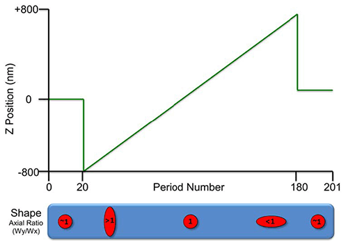
Figure 1449. N-STORM z calibration
The calibration steps are: collect 20 periods at the starting (in focus) position, move piezo to -800 nm at period 21, step piezo up in 10 nm increments to +800 nm, return piezo to starting (in focus) position for final 20 periods. The cylindrical lens changes the image of molecules' axial ratios as a function of z. The sequence can be performed simultaneously for all three reporter wavelengths (total of 603 frames).
Connect the Mad City Labs Nano-Z100 piezo stage to the PC via USB only (no more analog connectors). In case the MCL NanoDrive module is installed make sure to go to Devices > Device Manager and disconnect the MCL NanoDrive module. Otherwise the piezo stage will not move.
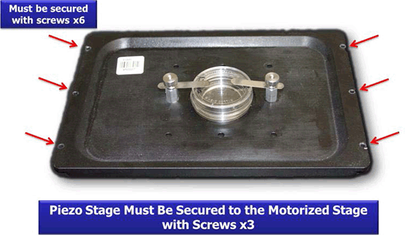
Figure 1450. Properly mounted calibration sample
The setup for calibration with 35 mm glass bottom dish is shown. Other sample vessels and holders can be used, but must be secured similarly.
Make sure the insert is securely mounted to the piezo by the 6 small screws, then turn the unit on. Place the calibration sample on the stage and secure it with clips (figure above).
Insert the cylindrical lens.
Focus on the beads using any of the reporter wavelengths. Identify a field with a dispersed, uniform distribution of beads within the 256x256 region used for STORM. Avoid sparse fields and bead clumps (if beads are too close they will overlap when elongated which can lead to miss localizations).
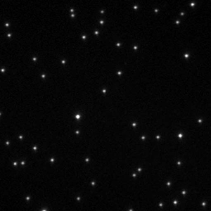
Figure 1451. 100 nm Tetraspeck bead field
A good 256x256 pixel field has a sufficient number of beads which are evenly distributed. There are few clumps or overlapping beads.
Setup the desired reporter wavelengths by clicking on in the N-STORM with the Agilent Acquisition window. Label the three reporter channels and select the appropriate lasers (figure below, red boxes). The color for displaying localizations in each channel can also be set here. If a laser is not selected as reporter wavelength it will not be available in the Z-calibration dialog (see the next step).
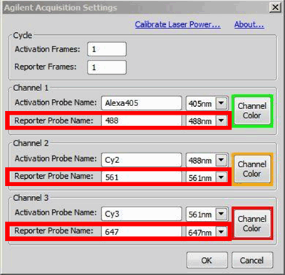
Figure 1452. Setting up the channels and lasers for calibration
Label and select the appropriate lasers here. Cycle settings and activation probes are ignored for calibration. Also, 405 nm is not used as a reporter and cannot be calibrated.
Click “Z Calibration” in the N-STORM with the Agilent Acquisition window (figure below, left). The window will change to calibration mode (figure below, right) and the piezo will immediately home to the center of its range. You will therefore have to refocus by moving up 50 µm.
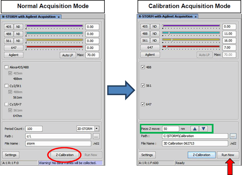
Figure 1453. Calibration settings
Acquisition dialog is switched to calibration mode by clicking “Z Calibration” (left, red circle). The reporter wavelengths to be calibrated are checked and path/filenames specified. button begins the calibration routine outlined in the “N-STORM z calibration” figure.
Check the boxes corresponding to the reporters to be calibrated, and specify the path and name of the calibration file (figure above, right).
As a final step, go live using the camera and refocus on the beads. Adjust laser power to give a good signal to noise ratio in each channel. Also check for the out of focus levels where the beads are elongated. At the same time you should avoid saturation in the in-focus frames. Use the “Piezo Z move” arrows (figure above, green box) to set the step size and fine tune focus with the piezo. The goal is to get beads as round as possible (axial ratio ~ 1). Zooming in helps in this regard.
Press to acquire the calibration (figure above, red arrow).
Connect the Mad City Labs Nano-Z100 piezo stage to the PC via USB only (no more analog connectors). In case MCL NanoDrive module is installed, make sure to go to Devices > Device Manager and disconnect the MCL NanoDrive module. Otherwise the piezo stage will not move.
Figure 1454. Properly mounted calibration sample
The setup for calibration with 35 mm glass bottom dish is shown. Other sample vessels and holders can be used, but must be secured similarly.
Make sure the insert is securely mounted to the piezo by the 6 small screws, then turn the unit on. Place the calibration sample on the stage and secure it with the clips (figure above).
Insert the cylindrical lens.
Focus on the beads using any of the reporter wavelengths. Identify a field with a dispersed, uniform distribution of beads within the 256x256 region used for STORM. Avoid sparse fields and bead clumps (if beads are too close they will overlap when elongated which can lead to miss localizations).
Figure 1455. 100 nm Tetraspeck bead field
A good 256x256 pixel field has a sufficient number of beads which are evenly distributed. There are few clumps or overlapping beads.
Setup the desired reporter wavelengths by clicking on in the N-STORM window. Select Multi-color Continuous Mode and label the three reporter channels and select the appropriate lasers (figure below, red boxes). The color for displaying localizations in each channel can also be set here. If a laser is not selected as reporter wavelength it will not be available in the Z-calibration dialog and if it is not labelled correctly it will appear wrong in the z-calibration dialog (see the next step).
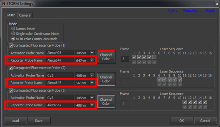
Figure 1456. Setting up the channels and lasers for calibration
Label and select the appropriate lasers here. Cycle settings and activation probes are ignored for calibration. Also, 405 nm is not used as a reporter and cannot be calibrated.
Click on in the N-STORM window and then on in the panel that appears below (figure below, left). Select 3D STORM. The window will change to calibration mode (figure below, right) after a message that will ask you to put in the cylindrical lens, the piezo will immediately home to the center of its range (you will therefore have to refocus by moving up 50 µm) and all the lasers go to 0% while a live window appears. For refocusing select one laser channel and set the laser power to 5-10%.
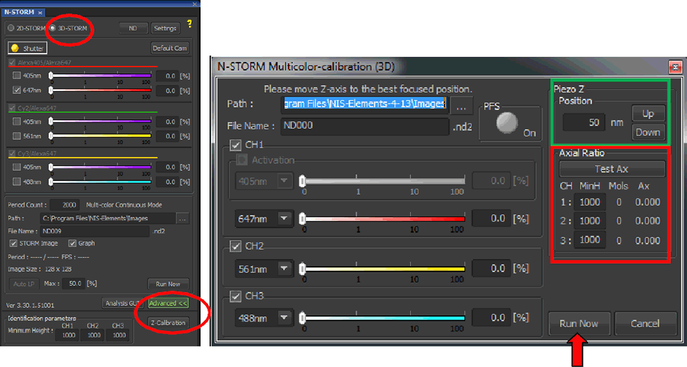
Figure 1457. Calibration settings
Acquisition dialog is switched to calibration mode by clicking (left, red circle). The reporter wavelengths to be calibrated are checked and path/filenames specified. button begins the calibration routine outlined in the “N-STORM z calibration” figure.
Check the boxes corresponding to the reporters to be calibrated, and specify the path and name of the calibration file (figure above, right).
As a final step, adjust laser power to give a good signal to noise ratio in each channel. Check for this also out of focus levels where the beads are elongated. At the same time you should avoid saturation in the in-focus frames. Use the “Piezo Z move” arrows (figure above, green box) to set the step size and fine tune focus with the piezo. The goal is to get beads as round as possible (axial ratio ~ 1). For the fine adjustment you can use the Axial Ratio test tool (figure above, red box and snapshot below). By pressing the N-STORM Graph Ax window opens up. You can see the live axial ratio for all selected colors. By selecting the range and the Auto Scroll period number you can adjust the graph. Bring the axial ratio of all colors as close as possible to 1 by moving up and down with the piezo (red box in the figure below). The differences you can see between the colors are due to chromatic aberrations that can be corrected later on.
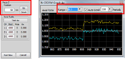
Figure 1458.
Press to acquire the calibration (figure above - Calibration settings, red arrow).
Open the N-STORM Analysis Module and load the calibration ND2 file.
Set the Identification S6ettings (figure below, left - Identification of beads for 3D calibration) for each channel low enough that beads are picked up in the out of focus frames. It is important to realize that in order to get a calibration of +/- 400 nm around focus only the most central 80 frames are needed (figure below). In these 80 frames it is important to get as many but also as reliable identifications as possible. Therefore, you should select a frame between 40 and 50 and base your identification settings on this frame. Make sure that you get around 50% of the beads identified. Recheck your settings on frame 160. Also here you should have around 50%.
Figure 1459. Reasonable calibration
Finally, check your settings on frame 60, 100 and 140. In these 3 frames you should get as many beads identified as possible and as little false positive as possible. Use the “Test” function to confirm this for all channels prior to running the analysis (figure below, right). Run a 3D analysis (figure below, red arrow) of the calibration data.
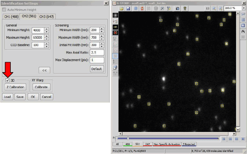
Figure 1460. Identification of beads for 3D calibration
Select the minimum height for each channel. In this example, a minimum height of 4000 for the 561 channel (left) results in identification of molecules in period 21 (right), corresponding to a z position of -800 nm.
To z calibrate, click on in the Identification Settings window (figure below - Generating the z calibration, red arrow). By pressing the button in the Z-calibration dialog and then holding shift while selecting Axial Ratio vs. Period (frame average) a graph will pop up that will show the changes in the axial ratio as function of frame number of all acquired channels (up to 3, figure below, lower panel). Use this graph to judge if the calibration will be OK. Please check for this if the (almost) linear behavior of the curves covers a range of at least 600 nm (in the case below it is around 800 nm, from frame 60 to 140 = 8 frames of 10 nm steps = 800 nm).
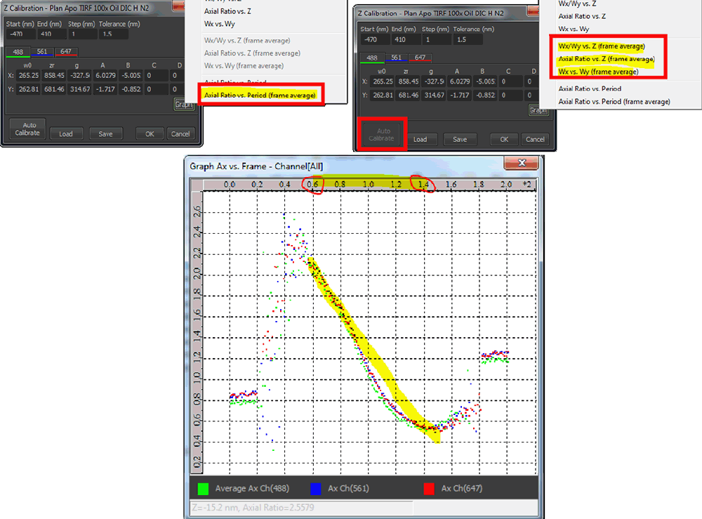
Figure 1461. Judging the quality of the Z-calibration data
If correct, press in the Z Calibration window (figure below, green arrow). There is a pause while the calibration is generated, after which the button is grayed out. New values and graphs will populate the dialog if calibration is successful (figure above, top right panel). The software automatically sets the range of the calibration depending on the quality of the data (figure below, red box). The difference between start and end point should be in the range of 600-1200 nm. Usually it will be around 800-900 nm.
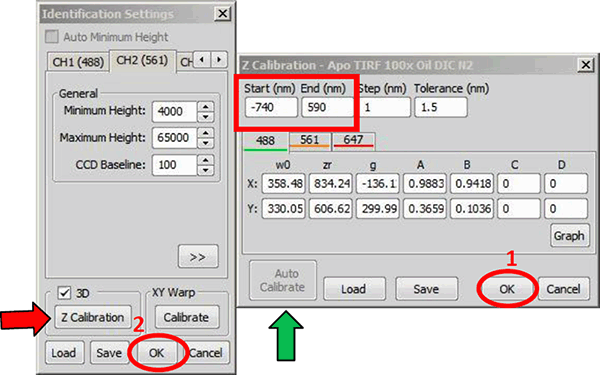
Figure 1462. Generating the z calibration
The Z Calibration window on the right is opened through the Identification Settings window (red arrow). Pressing (green arrow) calibrates the system. Clicking and again applies the calibration to the system.
If the calibration fails, the following error message will pop up.
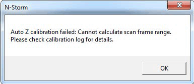
Figure 1463.
In the location where your acquired z-calibration file is stored you will now find a file with time and date as file name with the ending .log. At the very bottom of the file you will find an error message. Please see the Error messages during 3D calibrations chapter for the meaning of different error messages and to find suggestions how to avoid the errors.
If successful, evaluate the result of the calibration by checking the newly accessible calibration graphs (see typical graphs below). Note they are only available right after performing the auto calibration. The Z-calibration graph should display two crossing curves as shown below. Ideally the fitted yellow and blue curves are symmetric. Adjusting the correction collar may be needed if the curves are not symmetric. The axial frame average vs. z position graph should show a linear behavior over the central 800 nm (see example below). Any back curling should be avoided. If starting and end points should be around aspect ratio of 1. If they are far off (like in the shown example) please rerun the calibration and focus the starting point better. Finally, the average per frame of Wx vs. Wy should show a c-like shape. Again back curling should be avoided by all means. These three types of graphs are separately available per channel of the calibration data.
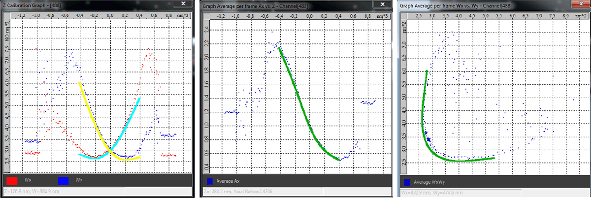
Figure 1464.
If the results are not satisfactory, press to revert back to the original calibration. To accept and apply the new calibration to the system must be clicked twice, first in the Z Calibration window then in the Identification Settings window (figure above - Generating the z calibration). Please see the N-STORM Analysis help file (see N-STORM Acquisition and Analysis) for a description of the parameters displayed at the end of calibration and description of calibration graphs.
After z-calibration is complete, you can now correct for chromatic aberrations, using the same data set. For this click under XY Warp in the ID Settings window (figure below, yellow arrow). A window opens displaying the result of the warp (figure below, right). Click to apply the 3D Warp to the system. This step can be skipped if the warping will not be used.
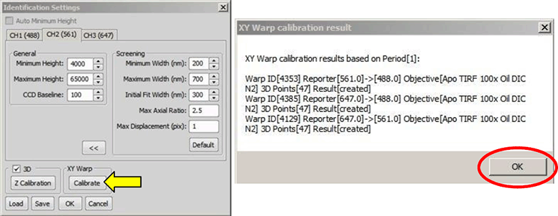
Figure 1465. Calibrating the system warp
Clicking “Calibrate” (yellow arrow) calculates the warp. The result window (right) opens when the warp is successful.
The cylindrical lens introduces a small distortion to the image. For this reason, it is necessary to generate a separate warp if channel registration is to be corrected for 2D experiments collected without the cylindrical lens. The workflow is similar to the steps described above for 3D, and is summarized below.
Remove the cylindrical from the light path.
Bring the beads into focus with the piezo and collect a calibration file for all channels to be warped as in steps 3-8 above. Note, that there will be no asymmetric stretch of beads without the cylindrical lens but the beads will blur instead.
Open and analyze the calibration file, this time using 2D analysis parameters (figure below). Also you should choose your identification settings depending on an in-focus frame (one of the first or last 20 frames of the acquisition or around frame 100 of the acquisition. These are the frames that should be in focus). As the 2D warp calibration only has to correct in 2D the warp correction is based on the frame where the beads are best focused (axial ratio closest to 1). Therefore, the identification settings can be more strict than in the 3D case where also out of focus beads need to be fitted.
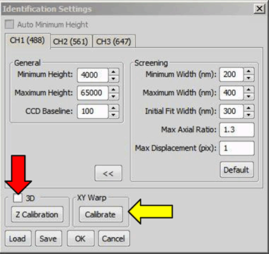
Figure 1466. Analysis for 2D warp
By unchecking “3D” in the Identification Settings window (red arrow), screening parameters are changed for analysis of 2D experiments collected without the cylindrical lens.
Click under XY Warp (figure above, yellow arrow). A warp for 2D is generated and a window opens displaying the result of the warp (figure below). Click to apply the 2D Warp to the system. This step can be skipped if warping will not be used.
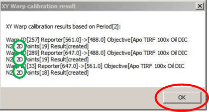
Figure 1467. 2D warp result
Note that the window now specifies that the 2D warp is generated (green circles).
The z-calibration algorithm automatically judges how good the acquired data of the z-calibration data file is. The quality of the data set depends both on the quality of the acquisition but also on the quality of the analysis. Thereby, selecting strict identification settings for the analysis of the z-calibration dataset can result in a better calibration curve.
In the following section the checkpoints and the criteria that the software applies are described. You will also find some suggestions how to resolve the situation if you get error messages following a failure at one or the other checkpoint. Note that only the first criterion that fails will generate the error message. Therefore several improvement steps might be needed before a calibration succeeds.
What are the criteria the software uses to judge if the z-calibration is OK or not:
Let`s have a look at the average per frame graph of a rather good (almost ideal) calibration data set. Vertical axis is the average per frame axial ratio. The horizontal axis is the period number (or for a single channel acquisition). The points (A, B, C, D, E, F, G) will help to define the constraints.
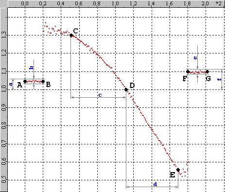
Figure 1468.
The first 20 frames of a z-calibration are acquired near the focal plane (data between points A and B on the graph). It is called the “first plateau”. Similarly the “second plateau” is the last 20 frames (data between points F and G). All points between B and F are acquired during the piezo scan in the middle between the two plateaus. In the scan extremes (between B and C and between E and F) optical aberrations are often so bad that the data is highly distorted (for example Airy disks or bad noise, etc). These two regions are called “garbage” and the software tries to exclude them from calculation.
The points between C and E form a nice curve that is easy to follow and fit. Somewhere in the middle of that region there is point D where the axial ratio is closest to 1.
The small blue letters in the graph (a, b, c, d, e, f) represent the following constraints:
Figure 1469.
The vertical position of every point between A and B must be within the range of 0.625 < a < 1.6 (note: 1 / 1.6 = 0.625).
The vertical range of the points between A and B must be less than 0.1 to avoid a warning and less than 0.2 to avoid an error.
It must be at least 30 frames which equals 300 nm.
It also must be at least 30 frames.
For multichannel acquisitions, each channel is evaluated independently. As you can imagine, satisfying all these requirements gets more difficult when:
you do 3 channels at once (because of chromatic aberrations),
you have an imperfect objective with asymmetrical PSF,
you start your acquisition far from the focal point,
you have excessive drift or vibrations,
piezo is not working properly.
Possible error messages:
Error! Channel[1 - Alexa 647] one of detected scan edges[58 120] is closer to detected midpoint[95] than min[30]
The horizontal (frame) position of your point C was 58, E was 120, and D was 95. Therefore D was not far enough from E (25 only instead of the required 30). Therefore criterion d is violated. A similar effect could happen for point C and criterion c.
Solution: Your starting point is probably not well focused. If you start your calibration at an out of focus position the midpoint (axial ratio =1) will not be centered. Alternatively, your piezo might not move linearly.
Error! Channel[1 - 647nm] Average Ax Range[0.202741] is above tolerance [0.200000]
The flatness of the first plateau is not good enough. The variation in axial ratios during the first 20 steps is too high. Criterion b (or e) is violated.
Solution: Check if your sample is well clamped. Also check if the anti-vibration works properly or if there is any other reason for vibrations (e.g. camera or other instrumentation on the system, air draft, construction work, etc.). Finally, also check if the beads on your sample are not floating and that all beads are in the same focal plane.
Warning! Channel[1 - 647nm] Average Ax Range[0.102741] is above tolerance[0.100000]
Same as error number 2 but this time only a warning is displayed. It means that your calibration is OK but you should check if there is a way to improve the situation.
Error! Channel[1 - 647nm] Min[1.000000] or Max[1.620727] Average Ax in starting plateau is outside of tolerance range[0.625000 - 1.600000]
One or several of the points in the first plateau is outside the tolerance range. This leads to a violation of criterion a (or f in case of the second plateau).
Solution: Check if you start the z-calibration procedure in an in-focus position. If the starting plateau is OK but the end plateau not, you are most likely suffering from a drift. Please check if you sample is clamped well, that there is no airflow on the system and that there are no temperature fluctuations. Also check that frame averaging is disabled. Finally, make sure that the beads in your sample are not floating and that all the beads are in the same focal plain.
Beads aggregate during storage. They must be vortexed or sonicated before and after diluting to ensure a good distribution on the coverslip.
Beads for calibration are imaged on the surface of the coverslip throughout the range of calibration. Therefore, the imaging medium has a negligible effect on the optical path length (spherical aberration) and imaging beads in air is acceptable. Calibration can be performed in water, but care must be taken that beads are not floating (which creates non-uniformity in axial ratios for a given z position).
Check that the piezo controller is connected to the PC by USB and turned on and that the MCL NanoDrive module is disabled (if applicable) under the Manage Devices settings. Also, very long USB cables sometimes cause communication issues for the Nano-Z100 controller. A short cable may restore piezo movement in this instance.
Make sure the cylindrical lens is in. If there is still no stretch, adjust the correction collar (turning it clockwise usually increases stretch, at the cost of enhancing optical aberrations that can hurt calibration). See the following question “Can I backup my z calibration” for more information on the correction collar.
Enough to generate good statistics, while at the same time avoiding clumps and/or overlap. This is usually accomplished with 25-100 beads in the 256x256 pixel region.
A warp is a non-linear transformation of one channel with respect to another. This means the registration shift is different throughout the field. The same beads are imaged with different wavelengths to act as fiducials mapping the registration offset between channels. To help ensure that the entire field is sampled a minimum of 10 beads must be successfully identified in both channels that are mapped to each other (there a three warps generated; 647 to 488, 561 to 488, 647 to 561). Lowering identification settings often results in more matching pairs. If the calibration still fails, move to a different field.
Earlier versions of the N-STORM analysis required max displacement set to zero and drift correction manually turned off by the user for calibration, and then turned back on for experimental data. Analysis modules with N-STORM with Agilent version 1.0.9 and later (analysis module b85 or higher) recognize calibration files and automatically set these parameters.
Yes, you can. The z calibration can be saved as a text file. It is highly recommended to save a backup copy of the current system calibration with your original data. This text file is also useful to move calibration to an offline workstation. The calibration is saved and re-loaded through the Z Calibration dialog (figure below).
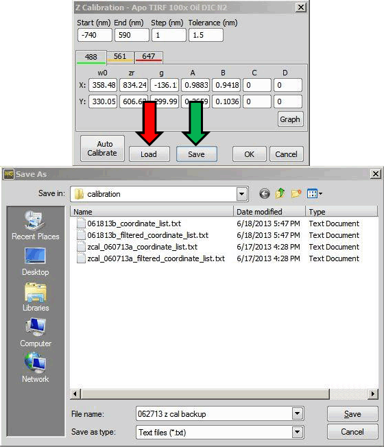
Figure 1470. Saving and loading z calibrations
Click (green arrow) in the Z Calibration window to save the calibration as a text file. A saved calibration is re-loaded by clicking (red arrow). It is necessary to click twice.
If your N-STORM system is equipped with a 100x 1.49 NA TIRF objective it will have a correction collar. The position of this collar has a large impact on the z calibration. Generally, the position for 23 ºC, 0.17 mm coverslip thickness is a good place to start. The collar should be set such that there is pronounced stretch in the molecules when they move out of focus. At the same time, it can be used to offset optical artifacts. These typically appear as holes in the diffraction limited spots at the extreme out of focus range (around -800 or +800 nm, figure below). The goal of collar adjustment is to maximize molecule stretch while minimizing the appearance of these holes, which will cause a reversal in the measured axial ratio and decrease system calibration range.
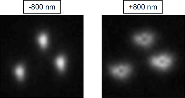
Figure 1471. Molecule shapes and aberrations during z calibration
Zoomed and cropped images of beads from opposite ends of a z calibration. At the -800 nm piezo position, the molecules appear stretched vertically with no significant aberration. Holes resulting from optical aberration are observed at the +800 nm piezo position. Correction collar adjustment can help balance the stretch and aberration.