Depending on the computer processing power and the amount of data STORM analysis may take a long time to complete. To facilitate processing of large amount of raw data N-STORM analysis software provides the capability to process multiple data sets in automatic unattended mode (typically overnight). User can create a list of data sets with their associated identification parameters and perform their sequential analysis. Batch processing is configured and launched from the Batch STORM Analysis dialog window.
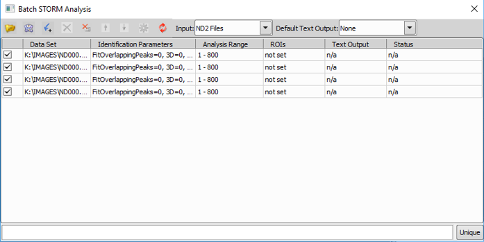
Figure 1419.
 Load SBDx
 This button opens a standard Windows Open File dialog allowing the user to open a batch job file.
 Save SBDx
 This button opens a standard Windows Save File dialog allowing the user to save the batch job file into the specified folder with a specified name.
 Add current ND2 as task
 This button inserts a new task line. The task line is populated with an ND2 file path, ID parameters, and selected period range currently set in the main dialog.
 Delete selected task(s)
 Deletes the selected tasks.
 Delete all the task(s)
 Deletes all tasks.
 Move selected task(s) up
 Moves the selected task(s) up.
 Move selected task(s) down
 Moves the selected task(s) down.
 Edit Identification parameters for selected task(s)
 Opens the Identification Settings dialog used for this input (please see Identification Settings).
 Start Batch Analysis
 Executes the batch job. Once the job is executed, this button changes to Terminate Batch Job so that the batch job can be stopped.
Only the selected file type can be added to the list of tasks.
Sets the default text output.

Each row corresponds to one task. If this option is checked, the selected task is included in the current job.
Shows the file system path to the raw data set associated with each task. Double-clicking on the data set name opens the selected source image.
Shows identification parameters for each task. Double-click on the parameters opens the Identification Settings dialog window used for adjusting the parameters (please see Identification Settings).
Displays the period (or Time slice for Live Cell data) range for each task.
Displays any available ROI(s).
Specifies the optional text output format.
This column is active only when the batch job is running. It displays the status of each task. For the tasks that have not yet started it is blank. For the currently active task it displays the percentage progress of each step. For processed tasks the status can be “Completed” or “Terminated” or “Failed” for STORM Analysis tasks, or number of molecules output for Molecule List Conversion tasks. Some of the common failures have specific descriptions such as “Failed to load” or “Failed to Identify”, etc.
Processing of a single data set is called a Batch Task. One or more Batch Tasks combined are called a . The Batch STORM Analysis dialog represents one batch job and has a list of its tasks. There are two basic types of batch tasks:
STORM analysis.
Molecule list conversion (generates one or more text molecule lists from the binary molecule list).
Each row in the list corresponds to one task. The check boxes in the left column control inclusion and exclusion of their corresponding tasks in the current job. The second column contains the file system path to the raw Data Set associated with each task. The third column holds Identification Parameters (such as CCD Background, Min Peak Height, etc.) for each task. The Analysis Range (or Time slice for Live Cell data) for each task resides in the fourth column. The third and fourth columns are not applicable to Molecule List Conversion tasks. Fifth column is used to specify the optional Text Output format. The last (sixth) column is active only when the batch job is running. It displays the Status of each task. For the tasks that have not yet started it is blank. For the currently active task it displays the percentage progress of each step. For processed tasks the status can be “Completed” or “Terminated” or “Failed” for STORM Analysis tasks, or number of molecules output for Molecule List Conversion tasks. Some of the common failures have specific descriptions such as “Failed to load” or “Failed to Identify”, etc.
Text output format column
This column for a newly added task is set to “Default”. In this mode, the global Default Text Output at the top right of the Batch STORM dialog window is applied.
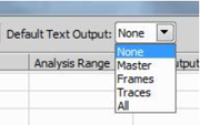
Figure 1420.
Each task can have independent setting by specifying Text Output options other than Default as shown below.
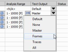
Figure 1421.
Multiple tasks can be selected and applied the same Text Output option also.
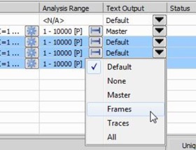
Figure 1422.
To Add a STORM analysis task, load a data set, adjust the identification parameters, set the analysis range, and then use the toolbar button. This should add a new row to the list of tasks and copy the current combination of the file path, identification settings, and analysis range. Alternatively one or multiple ND2 files can be dragged and dropped onto the Batch STORM Analysis window from Windows Explorer. Files which have identification settings embedded show up as batch tasks with those settings. Newly acquired files inherit the current system set of identification settings.
The input for STORM analysis task is an ND2 file. The output of STORM analysis task is a binary molecule list. The input of molecule list conversion task is a binary molecule list. The output of the molecule list conversion task is a text formatted molecule list. STORM analysis task can optionally produce text molecule list in addition to unconditionally produced binary molecule list. To add binary molecule list conversion tasks drag and drop one or more binary molecule list files from Windows Explorer to the Batch STORM Analysis window. STORM analysis and molecule list conversion tasks can be mixed in a single batch job. Adding tasks via drag and drop also supports folders. When a folder is dropped onto the Batch STORM Analysis window it is searched for all ND2 files (extension .nd2) and binary molecule lists (extension .bin).
The Input drop down list works as a filter during folder or multi-file drag and drop operations. It can accept only ND2 files, or only binary molecule lists, or both.
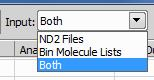
Figure 1423.
Select the desired option before adding tasks using drag and drop. If the set of files being dropped contains only one type of files (for example only molecule lists) but the input filter is set to only accept the other type (ND2 files for this example) then, as a convenience feature, the filter is ignored and the dropped files are accepted as batch tasks.
The task list supports common Windows multiple item selection behavior using Shift or Ctrl. Highlighted tasks as a group or individually can be moved up and down the list ( ) or deleted (). To quickly clear the job, all tasks can be deleted at once (). While batch job is in the setup mode (not running) the main STORM dialog is accessible and can be used to configure individual tasks (one at a time). To edit an existing task user can use the toolbar buttons. The button loads the tasks data set, identification parameters, and analysis range into the analysis module. The button facilitates editing of identification settings for the corresponding task. The same button on the toolbar edits identification settings of the first highlighted task. Once clicked, it brings up a standard Identification Settings dialog (Identification Settings) pre-populated with values pertaining to the task.
Default Text Output is optional for STORM Analysis tasks and mandatory for binary molecule list conversion tasks.
The entire batch job can be saved into and loaded from a file using and buttons that open standard Windows Open File and Save File dialogs with file filters set for STORM Batch Data (*.sbd) files. A STORM Batch Data file can also be dragged and dropped onto the Batch STORM dialog to open.
Use the button to execute the current batch job. Once the batch job is active, the main Batch STORM Analysis dialog becomes unavailable until the batch is stopped or finished.
While the batch job runs the molecule lists are saved in the same directories with their respective ND2 data sets. To avoid file naming conflicts the molecule list file names are suffixed with the time stamp at the time when each is saved. This is the default behavior. It can be changed to one of the behaviors by clicking on the status bar right pane (unique/overwrite/rename old).
Output Molecule List File Name Format
To avoid file name conflict, molecule list files saved by the batch processing have the following format:
<ND2-file-title>_list-<Timestamp>_S<#>.bin
where:
<ND2-file-title> is a data set ND2 file name without the extension (.nd2)
<Timestamp> is the date and time when the batch job is started (e.g. 2019-01-30-13-45-05)
<#> is the row number in the task list (1~)
This dialog window is used for creating a custom raster document from the currently opened molecule image.
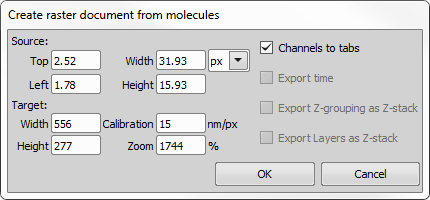
Figure 1424.
Set the source area to be exported either by entering the Top/Left/Width/Height values or simply by repositioning the red rectangle in the image. Make sure proper units are selected.
Set the target size (Width/Height) of the image being created and optionally set its calibration and zoom (image magnification).
If multiple channels are present in the image, the created document will have each mono channel as a separate tab. If this option is not checked, a RGB image will be created.
Turn on Show Conventional Image in the STORM Display Options dialog.
In the N-STORM window, move the Period Slider to the middle of the dataset.
Make sure an activation frame is not currently being displayed. If so, move the frame slider to an imaging frame.
In most cases the correct CCD Baseline value will be automatically determined based on the camera model. N-STORM analysis software displays the CCD Baseline edit field only when it fails to find the correct value. In that case enter correct CCD Baseline value for the camera used to acquire the raw data. It can be evaluated by looking at the average pixel intensity in an image captured without any light striking the camera sensor.
Hover the mouse over the candidate PSF peaks. Look at the status bar to see the intensity under the mouse cursor.
Find representative intensity peaks in the image and determine the relative peak intensity and the local background intensities around each peak. Subtract the local background from the central peak.
Repeat Step 6 for a few peaks over several images to find the smallest (Min. Height) and largest (Max Height) relative peak heights that should be considered molecules.
The procedure above assumes that the user is looking at the Status Bar to view the intensity of the pixel it is currently hovering over.
The Identification Settings dialog is the first and most important step to making sure that the STORM Image is properly created. This section (and subsequent sections) is an explanation of each setting and suggested values or methods to determine the correct values.
Check this box to perform automatic min height detection during analysis. When auto min height is selected the software runs a short (100 periods in the middle of selection range) pre-analysis with relaxed identification constraints to determine the optimal min height for a given data set. This feature is not available when a Z Calibration data set is loaded.
Check this box to allow fitting algorithm consider variable number of pixels depending on width and axial ratio of each individual peak. When this check box is cleared a fixed size pixel rectangle (typically 5 x 5 pixels) is used for fitting. Auto Fit ROI is recommended for 3D analysis. Fixed size ROI is recommended for 2D analysis.
The intensity of the smallest (dimmest) peaks (minus the local background of that peak) to be identified as molecules. Any object whose peak intensity is below this value will not be identified. Please see Determining Min and Max Height. If auto min height feature is selected the Minimum Height displays “auto” until the N-STORM analysis is performed at which point the “auto” is replaced with the actual calculated min height value.
The intensity of the largest (brightest) peaks to be identified as molecules. Any object whose peak intensity is above this value will not be identified. Please see Determining Min and Max Height.
Closed shutter (zero photons) pixel response. For Andor DU897 and for Hamamatsu Orca Flash 4.0 cameras it should always be 100. When currently loaded ND2 file was acquired with an officially supported camera, the CCD Baseline field becomes read-only and is automatically populated with the name of the camera manufacturer and the correct for the camera baseline value.
The smallest possible width a spot of some intensity in the image to be identified as a molecule by STORM Analysis.
The maximum possible width a spot of some intensity in the image to be identified as a molecule by STORM Analysis. A suggested default for 2D is 400nm. For 3D STORM, this should be slightly larger to take in account defocused molecules (above and below the focal plane). A suggested default for 3D is 700 nm.
This value is used as a starting point for STORM Analysis for identifying molecules. For 2D STORM, this is the expected value of a diffraction limited spot. A suggested default for both 2D and 3D is 300 nm.
Fluorescent spots whose ratio of elongation in the X and Y direction is larger than this threshold will be rejected as a single molecule. It is typically set to 1.3 for 2D STORM and 2.5 for 3D STORM.
This value sets the maximum distance (in pixels) that a molecule identified in one frame can be located from a molecule identified in the previous frame to be considered the same molecule and arising from the same Activation frame. The default value is 1. As mentioned in Z-Calibration section for Z Calibration files this value is ignored and 0 is used during STORM analysis.
This button can be used to quickly bring Max Width and Max Axial Ratio in correspondence with current 2D/3D status of the data. For 2D Max Width is set to 400 nm and Max Axial Ratio to 1.3. For 3D these settings are 700 nm and 2.5 correspondingly.
This checkbox indicates whether the dataset will be considered 2D or 3D during the analysis and subsequent display of results. This setting is typically applied prior to acquisition when the experiment is defined. During acquisition, it is stored to the ND file and read when the file is opened in the N-STORM module. However, this setting can be overwritten by checking or unchecking this box.
This check box selects the fitting algorithm used for molecule localization. When cleared, regular single Gaussian peak fitting algorithm is used. When checked, the software attempts to discover partially overlapping peaks and perform Gaussian fitting that accounts for such overlap. This algorithm generally produces better results with fluorophores whose blinking efficiency is less than that of Alexa647 (for example Atto488) or in densely labeled and over activated areas where molecule peaks tend to overlap in their respective frames. Algorithm that accounts for overlap may take longer time to compute. A reminder is displayed at the beginning of analysis (excluding Test) when Fit Overlapping Peaks is enabled. This reminder can be disabled for the session.
Drift correction is a process that looks at each frame of the dataset and correlates the amounts of drift that may have occurred over time. For 2D STORM datasets, only the lateral (X, Y) drift correction is performed. For 3D datasets, both the lateral and the axial drifts are corrected.
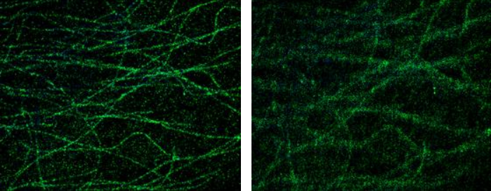
Figure 1425. Difference between Drift Corrected (left) and non-Drift Corrected (right) data
Drift correction is an automated process. It can be completed as part of STORM Analysis (check box in the STORM Analysis).
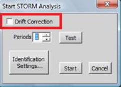
Figure 1426.
There are two types of drift correction. One uses the entire set of molecules to track the drift. This method is called Molecule Drift Correction. The other method (Bead Drift Correction) tracks registration fiducials (also called beads) attached to the cover glass. These beads fluoresce just like fluorophore molecules and their STORM localizations are attributed to dedicated “Drift Correction” channel. If STORM data set contains Drift Correction channel (set during acquisition), then by default the latter drift correction method is used. There is still an option to use the Molecule Drift Correction for drift correction if the data set is acquired as fixed cell however it cannot be used for drift correction in live cell data because the live cell molecule motion obscures the drift.
Bead drift correction depends on the quality of the captured bead data. Ideally there should be several beads that remain attached to the cover glass and visibly fluorescent in all bead frames. Also ideally extraneous beads should not float around beads tracked from the beginning, and molecule localizations should not appear near beads in the “Drift Correction” channel. In practice these conditions are not always met. The analysis software has a certain amount of tolerance built in it. All beads visible in the first bead frame are the candidates for tracking. Some of them may get disqualified as the tracking progresses. Disqualified beads are called “bad” and those that can be successfully tracked are called “good”. At the end of the bead drift correction “good” beads are marked with circles if ROI mode is enabled.
The center of the circle is a mid-point between the first and the last bead localization within each good bead trace. Diameter of the circle is proportional to the amount of drift at reasonably high zoom levels. In a relatively zoomed out view the circles have a fixed size. Otherwise they would be impractically small. Filter settings may exclude some bead localizations from the drift correction calculation, thus affecting qualification of the bead traces.
Color with Frame mode (also called Time Map rendering) is useful to visually evaluate bead traces. It can be toggled by the Ctrl+Shift+F key combination. Besides mapping the color to the frame number, for live cell data this mode shows all bead localizations at once (as opposed to single time slice worth of localizations as is normal for live cell rendering). Although Color with Frame mode can be used for other (non-bead) localizations, it is particularly useful for beads.
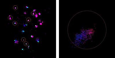
Figure 1427.
Ideally all the “good bead” traces should look similar. If certain bead traces look better (less spread) than others, then only those can be used as candidates for drift calculation. To do this, draw multi ROIs around good bead candidates, and then click the top toolbar button.
Even with manual bead selection the algorithm still evaluates bead quality and can reject some beads. In an extreme case all of the bead candidates may get rejected, which leads to a bead drift correction failure. When bead drift correction fails on fixed cell data set, autocorrelation method can still be used and is automatically offered.
Ideally, beads should be wavelength separated from the molecules. In other words, bead localizations should not show up in the molecule channels and the other way around. In practice this is often not true. N-STORM analysis software offers an option to hide bead localizations in the molecule channels. This is done by hiding all molecule localizations located within a small radius of bead localizations. The radius can be adjusted via “Phantom Bead Mols Search Radius” ini file variable. When data set with bead drift correction is loaded, “Hide Localizations near Beads” pop-up menu option becomes available.
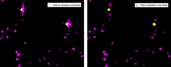
Figure 1428.
Hiding of molecules near beads can also be toggled via Ctrl + H, B sequence of keystrokes. After the initial Ctrl + H keystroke the window title displays one of the context sensitive reminder prompts below.
Each molecule in the text file will be listed on a separate line. Each line will contain the following pieces of information about that molecule:
Table 36.
| Field Name | Description |
|---|---|
| Channel Name | This is the name of the Channel where the molecule was detected. |
| X | The X position of the centroid of the molecule in nanometers. Similar to the conventional image, molecules positions in the image are relative to the upper left corner of the image. |
| Y | The Y position of the centroid of the molecule in nanometers. Similar to the conventional image, molecules positions in the image are relative to the upper left corner of the image. |
| Xc | The X position of the centroid of the molecule (in nanometers) with drift correction applied. If no drift correction was applied to this data then Xc= X. |
| Yc | The Y position of the centroid of the molecule (in nanometers) with drift correction applied. If no drift correction was applied to this data then Yc= Y. |
| Height | Intensity of the peak height in the detection frame (after the detection process). |
| Area | Volume under the peak. Units are intensity * pixel^2 |
| Width | Geometric mean of Wx and Wy.  |
| Phi | The Angle of the molecule. This is the axial angle for 2D and distance from Z calibration curve in nm in Wx, Wy space for 3D). |
| Ax | Axial ratio of Wy/Wx. |
| BG | The local background for the molecule. |
| I | Accumulated intensity. |
| Frame | The sequential frame number where the molecule was first detected. |
| Length | The number of consecutive frames the molecule was detected. |
| Index | Used in individual frame localization records only. Contains the index of corresponding linked molecule record. |
| Link | Index of localization in the molecule list of the frame pointed to by Frame field or -1 indicating the end of the trace. |
| Valid | For internal use only. |
| Z | The Z coordinate of the molecule in nanometers (origin is the cover glass). |
| Zc | The Z position of the molecule (in nanometers) with drift correction applied. If no drift correction was applied to this data then Zc= Z. |
| Photons | The total number of photons received from molecule across its entire trace length. This number is calculated using current (at the time of calculation) photons per count value. |
| Lateral Localization Accuracy | XY localization accuracy calculated using Thompson formula based on the number of photons. |
| Xw | X coordinate after XY warp transformation to compensate for chromatic aberration. |
| Xwc | X coordinate after XY warp transformation and drift correction. |
| Yw | Y coordinate after XY warp transformation to compensate for chromatic aberration. |
| Ywc | Y coordinate after XY warp transformation and drift correction. |
| Zw | Z coordinate after chromatic aberration correction Z offset has been applied. |
| Zwc | Z coordinate after chromatic aberration correction Z offset and drift correction have been applied. |
The following image illustrates the scheme used to link multiple localizations from adjacent frames into single molecule record.
Figure 1429. Molecule list with trace traversing structure.
Molecule list with trace traversing presents the molecule information rearranged for easy trace following. It is generally ordered by the master molecule list but the individual frame localization records are inserted immediately following the corresponding molecule record. Molecules with trace length of N will have N+1 records (master and N frames). For consistency molecules with trace length of 1 will have 2 identical records (master and one frame).
Table 37. Example of molecule records with trace length of 1. Mol[124939] count[1].
| X | Y | Xc | Yc | ... | |
|---|---|---|---|---|---|
| 111.21791 | 189.36948 | 111.70292 | 189.78879 | ... | (master) |
| 111.21791 | 189.36946 | 111.21791 | 189.36946 | ... | (frame 1) |
Table 38. Example of molecule record with trace length longer than 1. Mol[124944] count[3]
| X | Y | Xc | Yc | ... | |
|---|---|---|---|---|---|
| 206.68843 | 31.06892 | 207.17416 | 31.48837 | ... | (master) |
| 206.67001 | 31.07309 | 206.67001 | 31.07309 | ... | (frame 1) |
| 206.66777 | 31.00289 | 206.66777 | 31.00289 | ... | (frame 2) |
| 206.72476 | 31.13095 | 206.72476 | 31.13095 | ... | (frame 3) |
If any ROI(s) with molecules inside of them are present in your image, switch to the ROI Statistics tab to view the statistics per each ROI and for the whole image.
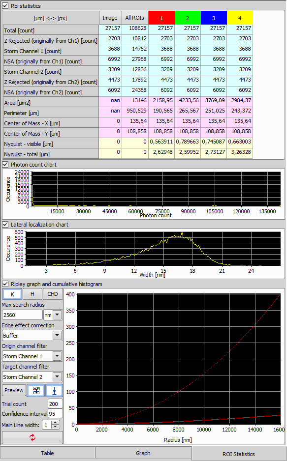
Figure 1430.
ROI Statistics Table
The table summarizes the number of molecules in the image and in all ROIs. If multiple ROIs are selected, their features are shown per each ROI (separate column). More features such as the area, perimeter, center of mass and Niquist are calculated as well. To easily switch the units used in the statistics, click on the button in the top left corner of the table.
The first graph shows the Photon count chart which represents the peak intensity histogram in the ROI.
The second graph shows the Lateral localization chart representing the Width of the Gaussian peak.
The third graph shows the Ripley graph and cumulative histogram. Select one of the three graphs for molecule population - Ripley's K function (K), Ripley's H function (H), or CHD and set the Max search radius and Border correction. All the three graphs use the XY distance between molecules as the horizontal axis.
For any given distance the value of the function is the number of molecule pairs in the ROI molecule population with distance equal or smaller to the given distance. Formal definition:
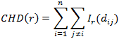
Figure 1431.
where I r I r is the indicator function defined as
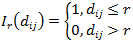
Figure 1432.
nn is the number of points
rr is the max neighborhood search distance around any given point
d ij is the distance between points i and j
Ripley’s K function is similar to CHD except it is scaled by factor:

Figure 1433.
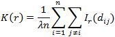
Figure 1434.
where λ is average density. In this form Ripley’s K function estimates the expected number of additional points within distance rr around a randomly picked point normalized per unit of density. λλ is the average density of the ROI population
λ = n/a
where aa is the ROI area.
Ripley’s K function is useful to explore cluster topology. When molecules form clusters, Ripley’s K function forms horizontal plateaus and steep rises (staircase look). For example, in the simplest case of two clusters, Ripley’s K function has one horizontal plateau.
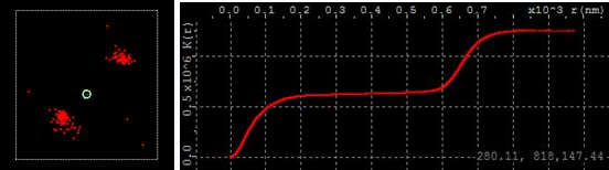
Figure 1435.
The horizontal axis of Ripley’s K function is the distance between molecules in a given pair. The vertical axis is proportional to the number of pairs in the population with distance not exceeding given. The first vertical rise on the left side comes from a number of close by neighbor molecules within each cluster. The position of the left edge of the horizontal plateau implies the size of clusters. As the distance increases further, the number of matching pairs does not increase until the distance reaches the distance between clusters. At that point the count begins to rise again, because larger distances between molecules of different clusters begin to contribute. Therefore the right edge of horizontal plateau suggests the inter cluster distance. Mouse cursor position in graph units is displayed in the bottom right corner as the mouse hovers over the graph area.
Ripley’s H function can be defined in terms of Ripley’s K function.
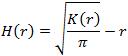
Figure 1436.
When points are randomly distributed, K function approximately follows the area of a circle function.

Figure 1437.
The K function exceeds area function, when data points form clusters on a given scale. Conversely, the K function falls below the area function, when data points disperse (or form voids) on a given scale. The H function makes detection of clusters (or lack thereof) easier than the K function, because its value remains 0 under CSR (complete spatial randomness) condition. When the data points exhibit clustering, the H function becomes positive and forms a visible peak. When the data points are distributed uniformly, the H function becomes negative.
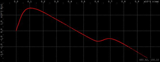
Figure 1438.
All three cluster analysis functions quickly become computationally expensive as ROI population grows. Calculation time is greatly affected by other options such as maximum neighborhood search radius and edge effect correction method discussed below.
Max search radius edit box below the function selection buttons displays and adjusts the max neighborhood search radius. The button on its right side provides (and cycles through) three choices for distance units: nanometers (nm), micrometers (µm), and pixels. Pixels correspond to the original camera pixels (typically 160 nm). The largest supported search radius is 16 pixels or approximately 2.5 micrometers. The units apply to both the max search distance and the graph. When units change, the value of the Max search radius edit box automatically converts. The choice of units does not affect the length of calculation, but, when changed, commences the new calculation rather than converting results of the previous one. Reducing the Max search radius can greatly reduce the length of calculation.
Border correction is an edge effect correction attempting to compensate for the lack of neighboring points when the search is conducted near the ROI border. The circular search neighborhood then partially falls outside of the ROI. None simply skips the correction. This is the fastest method. Perimeter implements the popular correction method based on the fraction of circle perimeter within the ROI. Each measured distance carries a weight factor. When the circle around point i with radius equal to distance to point j is completely contained in the ROI the weight factor is 1. Otherwise the weight factor is equal to the fraction of the circle perimeter within ROI and is less than 1.
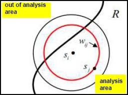
Figure 1439.
During Ripley’s K function calculation contribution of each distance is divided by its weight factor, thus increasing when weight factor is less than 1 and therefore compensating for the possibly reduced neighbor count.
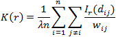
Figure 1440.
Perimeter based edge effect correction is the most computationally expensive. Switching to a faster method, if acceptable, can greatly reduce calculation time.
Border correction method simply counts neighbor points outside of ROI that fall within max search radius or ROI points, but does not search their neighborhoods. All weight coefficients remain 1.
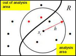
Figure 1441.
Edge effect correction applies to CDH and H(r) functions in a manner similar to K(r) shown above.
When molecule data has multiple channels, cluster analysis can be performed across channels. In other words the distances are measured in one direction: from molecules in origin subset to molecules in target subset. These subsets can be defined as all molecules or molecules belonging to one of the channels. All combinations are possible. For example a two channel data set provides the following options:
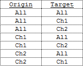
Figure 1442.
This button performs XY Warp calibration using the information extracted from the multi reporter Z Calibration file. This button is enabled only when such file is loaded and STORM analyzed. Since 3D Cylindrical lens can affect chromatic aberration and separate calibration is recommended for each combination of objective, reporter wavelength, and cylindrical lens. To calibrate 2D XY Warp acquire Z Calibration file without cylindrical lens in optical path. 3D XY Warp calibration can be achieved with regular Z Calibration file. Single multi reporter calibration file produces several calibrations at once (one for each wavelength except the shortest one, which serves as a base and does not require calibration). XY Warp is applied to molecule coordinates to compensate for the effects of chromatic aberration. Molecules with longer reporter wavelength can be optionally repositioned to locations where they would be likely to appear. This adjustment is necessary to correctly perceive the relative position between molecules reported in different wavelengths. Unsuitable beads can be manually excluded from the warp calibration by assigning multi ROIs around them.
Z Calibration is performed by analyzing a Z-Series dataset to determine the width and orientation of all identified molecules. Each Z Calibration pertains to an objective and an excitation wavelength. Objective name is displayed in the title of the dialog. Excitation wavelengths of different channels are presented as tabs in the upper half of the dialog. When data set (ND2 file) is loaded Z Calibration dialog displays only calibrations linked to the objective and the reporter wavelengths pertaining to the data. To view all known Z Calibrations maintained by the system (for other objectives and wavelengths) close current data set or restart the software and visit Z Calibration dialog when no data set is loaded. In this case two extra buttons allow iterating through the list of calibrated objectives. Individual reporter calibrations can be accessed via tabs named and colored after their respective wavelength. Additionally in this mode the and buttons at the bottom are renamed into Restore and Backup respectively and perform a different function that will be described below.
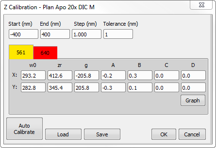
Figure 1443.
Wx-Wy vs. Z – This graph shows the Wx and Wy calibration curves (cyan and yellow respectively) and the identified molecule’s Wx (red) and Wy (blue) values that pertain to currently selected in Z Calibration dialog channel tab. Generally the number of raw data points is limited to 3000. To display all points hold the Ctrl key while selecting the menu item.
Ax Ratio vs. Z -This graph will show the ratio of Wy/Wx on the Y axis and Z on the X axis. It also shows the identified molecule’s Wy/Wx ratio values (in blue). Generally the number of raw data points is limited to 3000. To display all points from the currently selected channel hold the Ctrl key while selecting the menu item.
Wx vs. Wy – shows the plot of Wx vs. Wy for the calibrated curves (in green) and of the individual localizations from current channel (in blue). Generally the number of raw data points is limited to 3000. To display all points hold the Ctrl key while selecting the menu item.
Holding the Shift key while selecting this graph’s menu item displays the Z Rejected points in addition to the points from the currently selected channel tab. This helps checking how well the raw data follow the current calibration. Z Rejected molecules can be further categorized into those too far from the curve (yellow) and those with Z position beyond the calibration range (red).
Wx-Wy vs. Z (Frame Average) – this will show the same graph as above (#1) but only show the average Wx and Wy position per frame of the identified molecules. This graph is only available immediately after Z Calibration.
Ax vs. Z (Frame Average) - This will show the same graph as above (#2) but only display the average Ax (Wy/Wx ratio) per frame for the molecules. This graph is only available immediately after Z Calibration.
Wx vs. Wy (Frame Average) – This will show the same graph as above (#3) but only display the average Wx and average Wy per frame for the identified molecules. This graph is only available immediately after Z Calibration.
Axial Ratio vs. Period – This graph is useful for evaluating Z calibration data before performing Auto Calibration because it does not rely on any (previous or current) calibration. It simply displays the raw data points without any curve graphs. This graph is only available when Z calibration data is loaded and STORM analyzed. By default it displays up to 3000 points from the currently selected channel.
To display all points from the current channel hold Ctrl while selecting the menu item. Sometimes the data contains outliers that affect scaling. To exclude outliers and see the data that more closely resembles the filtered set used for actual calibration, hold the Alt key while selecting this graph’s menu item. This option picks only 80% of points from the middle of the distribution in every frame and rejects outliers.
To observe the effects of chromatic aberration on multichannel data hold the Shift key while selecting the menu item. This displays all channels at once.
The channel colors used in this graph match the pseudo colors of the calibration data set.
Axial Ratio vs. Period (frame average) – This graph displays almost the same data as the one above (#7). The only difference it calculates the average for every frame and displays it as one point per frame. It has all the same options (Shift for multi channel, Ctrl for all points rather than 3000, Alt for skipping outliers). This is the most useful graph to evaluate raw Z calibration data before actual calibration.
The software keeps track of multiple Z calibrations as they pertain to objectives with which they were acquired. During analysis the objective information is retrieved from the metadata and used to apply the correct calibration curves. If the calibration for data set objective is unavailable the software displays the warning and applies the default calibration. Similarly to Objective name software links calibration to reporter wavelengths and warns if calibration curve for any of the dataset wavelength is missing.
The objective name pertaining to current Z Calibration is displayed in the title bar of the Z Calibration dialog.
Calibrations for different wavelengths are affected by chromatic aberration. With a cylindrical lens in the optical path a given axial ratio of localizations happens at different Z positions for different wavelengths. Conversely a given Z position imaging with different wavelengths produces localizations with different axial ratios. When multiple wavelength calibrations are acquired and analyzed together, the software extracts axial chromatic shifts and maintains them along with calibration curves. When a newly acquired data set (acquired with the same objective and reporter wavelengths) is loaded and analyzed, the calibrated chromatic offsets are also applied to Z positions. The channel with the shortest reporter wavelength is used as a reference for chromatic aberration offsets.
All graph dialogs have pop-up menu options to change the color of the background and grid lines. These colors are shared by all N-STORM analysis module graph dialogs and persist across NIS-Elements sessions.
Similarly all graph dialogs share the ability to zoom by the mouse scroll wheel around the current cursor position and to pan the graph with a mouse drag operation.
Graph image as well as numerical data can be transferred to a third party application via Windows Clipboard or exported into an image or text files on a disk. Both options appear at the bottom of the right click pop-up menu.
All Z Calibration dialog buttons provide tooltip reminders.
These values specify the lower and upper Z limit of the calibrated dataset. Typically, these values will be smaller (by absolute value) than the top and bottom of the Z Stack used during the calibration process. These values are automatically updated during Auto Calibration.
This value specifies the resolution of the calculated Wx/Wy calibration curve. Typically, data points that make the curve are spaced 1 nm (in Z direction) apart from each other.
The tolerance value specifies how far from the  vs.
vs.  curve a molecule can be and still be considered valid. Any molecules that are further from the curve than the specified tolerance distance will be placed into a special channel called “Z Rejected”. Z Rejected Molecules can optionally be displayed. The Default tolerance value is 1.5 nm.
There are two ways to determine the Wx and Wy calibration curves. The first method is for the software to capture a special Z series of a calibration slide (sub-resolution beads mounted to the cover glass). The elongation of every molecule is measured and the software automatically generates the curves.
The second method is to use the data collected from the Z-Series dataset and calculate the calibration outside of NIS-Elements using third party analysis software. The coefficients that were calculated outside of NIS-Elements can then be input into the parabola coefficients for Wx and Wy.
The defocusing curve formula is:
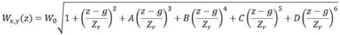
Figure 1444.
 is the lowest point in each graph
  or
or  .
.  and
and  should be approximately the same. If they are not, one parabola is positioned higher than the other. It means points focus tighter in one direction than in the other likely due to spherical aberration.
 is the focal depth of the microscope. Ideally it should also be the same between X and Y. Calibration fitting algorithm restricts it to stay below (and including) 5000.
 is the relative to focal plane Z position where each curve focused the tightest. Ideally the values for X and Y should be the same by absolute value but with opposite signs (X negative and Y positive). This would mean that calibration is perfectly symmetrical around focal plane.
and values can be directly found in the and  vs.
vs.  graph as illustrated below.
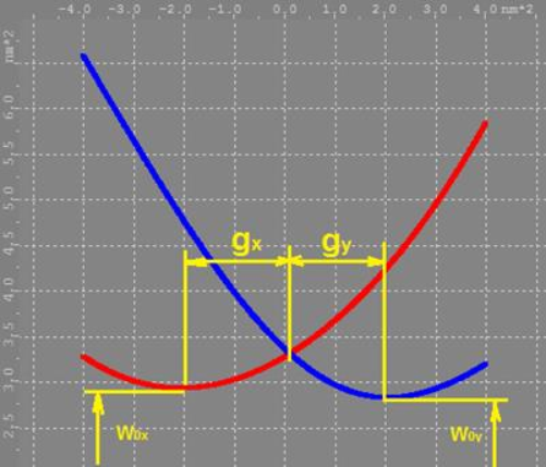
Figure 1445.
“A”, “B”, “C”, and “D” are higher order polynomial coefficients. A is the coefficient of the third order. B is the coefficient of the fourth order, and so on. Ideally all coefficients (A, B, C and D) should be 0. Typically coefficients A and B alone produce close enough approximation curve, so C and D are normally kept at 0 even in practice. There is an .ini file setting that removes the C and D constraint to deal with difficult cases. It's called “z calibration auto calib higher order corrections”. It is difficult to judge the quality of calibration by just looking at the values of these coefficients.
This button automates the process of creating the Z calibration curves. It requires a Z-Calibration molecule list present (loaded or analyzed). Holding Ctrl while pressing Auto Calibration button causes the algorithm to ignore high density cluster localizations that may lead to peak overlap in out of focus frames. Ignored localizations are reassigned to Z Rejected channel that is otherwise not used with Z Calibration data.
Z Calibrations can be saved to a text file. These files can then be opened and applied to other 3D STORM datasets. These buttons are only available when ND2 data set is loaded. They work with a subset of calibrations pertaining to current data set. These calibrations may be different from the calibrations maintained by the system for newly acquired data sets. Calibrations loaded in this manner are called “foreign”. They become active (in effect for the subsequent 3D STORM analysis) and temporary override system or embedded nd2 file calibrations. They do not overwrite system calibration, which goes back in effect as soon as current nd2 file is closed. Foreign calibration can be permanently embedded into an nd2 file if at any point after foreign calibration is loaded the nd2 file is saved.
This button displays the menu with options for various graphs that visualize calibration curves and raw data and help evaluate results of current Z Calibration. There are eight types of Graphs available.
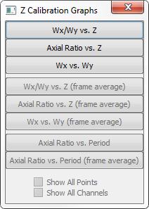
Figure 1446.
Some Automatic layer alignment algorithms involve examining and matching multiple ROIs. These ROIs can be defined manually or generated automatically. The mix of both is also possible. Click on the drop-down arrow next to the ![]() Start correlation button to open the Z-Stack Alignment Options.
Start correlation button to open the Z-Stack Alignment Options.
This section defines the set of ROIs to be used. Automatically generated ROIs are arranged in a grid with definable dimensions (Grid). The Mix Manual and Auto generated ROIs button controls the mixing behavior. When the button is unchecked ( )and manually defined ROIs exist, no auto generated ROIs are added. When the button is checked (
 ) or no manually defined ROIs exist, the grid of ROIs is generated according to grid dimensions. The left field is the number of columns and the right field is the number of rows.
Not all generated ROIs are good for layer alignment. Only ROIs that pass through the ROI filter are considered.
First ROI filter is by the molecule count  . ROIs with relatively small number of molecules are discarded. The Min Count threshold is defined as a percentage of the maximum single ROI molecule count among the ROI population. The button toggles the filter on and off. The filter is enabled by default.
The second filter is the Maximum average Nearest Neighbor distance filter ( ). If applied, it removes ROIs with average nearest neighbor distance greater than the specified percentage of the maximum average nearest neighbor distance if the molecules were evenly and randomly distributed throughout the ROI area without forming any structure or clusters. In practice this filter is not very useful because, with STORM, individual molecules get localized more than once. Even when fluorophores are evenly distributed, their localizations form tight clusters which significantly drives average nearest neighbor distance down, thus making ROIs that lack structure falsely identified as those containing a structure. This filter is available only in the mode and is disabled by default.
This group of controls provides several options that affect the autocorrelation algorithm input. Autocorrelation expects two similar signals. As it is used for layer alignment of localization data the signals are 2D density maps or histograms with bin values representing molecule counts falling within each spatial bin.
Z layer intersection ( )or union (
 )choice affects the Z position filtering during histogram build. Intersection is chosen by default.
Another option ( )is to merge ROIs for single autocorrelation and single offset result or (
 ) to perform separate autocorrelation for each ROI and then filter/average multiple results.
Outlier histogram bins can be optionally trimmed to avoid spurious autocorrelation offsets caused by occasional high density clusters. This option is enabled by default.

Figure 1447. 

Figure 1448. 
This filter is shown in the mode only. It is applicable to multi ROI alignment workflows that do not merge multiple ROIs (). This produces multiple offset results for a given pair of layers. The Offset Filter ( ) checks how well multiple Cubes agree on the XY offset. DBSCAN algorithm is used to find a cluster that pertains to the subset of cubes that well agree with each other. Offsets obtained from other cubes are then ignored as outliers. The good offsets are averaged. To troubleshoot difficult layer alignment the Test Mode is available via the
  button. In the Test Mode intermediate data from each cube autocorrelation operation is available for close examination and alignment offsets are not applied to layers.
Typical N-STORM Z calibration range is 800 nm (from 400 nm below to 400 nm above focal plane). Z stacking feature is available to overcome the 800 nm depth limit and image larger volumes. N-STORM acquisition module captures multiple slices along Z axis. Each slice covers the 800 nm Z range. Each slice raw data is stored in a separate ND2 file. To even out photo bleaching during acquisition, the volume can be acquired by spending shorter time at each slice while visiting each slice multiple times. In Z stacked STORM terminology the slices are also called “layers” and a set of unique layers is called a “pass”. The entire Z stacked STORM data set consists of one or more passes. Similarly to regular (non-Z stacked) 3D storm data, each layer has its Z position defined as the distance between the cover glass and the focal plane. The actual position of the focal plane is affected by spherical aberration. It is calculated by the software from the microscope Z mechanism displacement measured and stored in the ND2 file metadata. The displacement focal plane position (not the corrected one) is the one associated with each layer and displayed in the software.
Layers may overlap in the Z direction to aid alignment between adjacent layers and between passes. When they do, the focal plane positions of adjacent layers differ by less than the calibration range. Alignment is necessary to compensate for the drift during acquisition.
Z stack STORM ND2 files follow a file naming convention to preserve layer and pass numbering order. Each name is made of:
Base file name common to all files.
Pass number suffix that starts with letter P followed by two digit pass number (starting with 01).
Layer number suffix that starts with letter L followed by three digit layer number (starting with 001).
.nd2 extension.
Example 20. Example of two passes three layers Z stack with base name "Test_":
Test_P01_L001.nd2
Test_P01_L002.nd2
Test_P01_L003.nd2
Test_P02_L001.nd2
Test_P02_L002.nd2
Test_P02_L003.nd2
Similarly to the regular (non-Z stack) N-STORM workflow, ND2 files need to be analyzed to produce molecule lists that can later be rendered as super resolution images. Although each ND2 file can be analyzed individually, N-STORM Analysis module provides a simplified batch setup and processing to streamline the analysis of large amounts of data often associated with the Z stack STORM. Multiple ND2 files can be dragged and dropped onto the Batch window from Windows Explorer.
The molecule list files produced by batch analysis are named after their ND2 predecessors. The pass and layer index suffixes are preserved. To continue with the ND2 naming example above the molecule list files will be named:
Test_P01_L001_list-2015-08-07-10-45-20_S01.bin
Test_P01_L002_list-2015-08-07-10-47-30_S02.bin
Test_P01_L003_list-2015-08-07-10-49-40_S03.bin
Test_P02_L001_list-2015-08-07-10-51-50_S04.bin
Test_P02_L002_list-2015-08-07-10-54-00_S05.bin
Test_P02_L003_list-2015-08-07-10-56-10_S06.bin
Each molecule list can be loaded individually in a traditional way. To load and merge all layers at the same time simply drag and drop all pertaining molecule list bin files from the Windows Explorer onto the main N-STORM window. Multiple files can also be selected and opened at once via File > Open dialog using standard Windows (Ctrl and Shift) keys for multi file selection. Loading progress feedback is displayed in the window title.
One ND2 file can be loaded before multi file drag and drop operation or as a part of it. Multiple ND2 files and other non binary molecule list files are ignored if present among binary molecule lists drag and drop file selection. Skipping some of the layers (by excluding them from drag and drop selection) during load is acceptable.
The layers table in the Molecule Options dialog has the following main functions.
Displaying layer information
Selecting layer subsets for various operations
Setting up layer pseudo colors (automatically and manually)
Adjusting (ΔX, ΔY, ΔZ) layer offsets to align adjacent layers and passes (automatically and manually)
Toggling alignment offsets in rendered image
Multi ROI associated with layer subsets
Toggling between pseudo colors by layer and by channel
Layer information is displayed in a grid where each row represents a single layer.
Why do the molecules look dark when I am in Normalized Gaussian mode?
The most common cause is that the display properties for Normalized Gaussian are not properly set. It is common that molecules look bright when the image is near 1:1 because of the large concentration of molecules. However, when zooming into the image, they can tend to appear darker. Adjust the Min and Max Threshold in the Advanced Gaussian settings of the STORM Display Options dialog.
Why do I not see all of the molecules?
It is common that not all molecules will be displayed. The lower right hand Status bar will show how many molecules are currently displayed vs. the total number of molecules identified. Most likely, there are some filter settings in the Filter dialog that are currently selected. Note that some filters (like photon count and trace length) are in effect all the time and cannot be disabled. However, they can be relaxed to include a wide range of values.
How do I apply a Z Calibration to an already processed dataset?
After calibration, save the calibration settings to a text file (in the 3D Settings dialog). Open the processed dataset, and load this text file. Then perform STORM Analysis again. See section on STORM analysis workflow for more information.
When I turn on “Mark Identified Molecules”, only some yellow boxes have molecules inside. Why?
The Rel Frame Range filter was set and only molecules within that selected frame range are displayed.
Yellow boxes are always aligned to the low resolution image pixels. If you display drift corrected molecule positions the corresponding cross may be far outside the yellow box. In order to see it inside use uncorrected for drift coordinates.
There are some other filter settings that prevent the molecule inside the box to be displayed. Some filters cannot be turned off. For example minimum and maximum number of photons, and max trace length. If the number of photons per count is set incorrectly then some molecules could be pushed out of the allowable (to be displayed) range for the number of photons.
Yellow boxes remain on for the entire duration of the molecule trace. For example, if some molecule was first discovered in frame 1000 and remained fluorescing until frame 1005 (inclusive for the total of 6 frames) then the yellow box will be visible in all these frames. If you set your frame filter to only display molecules discovered in current frame (0 minus and 0 plus) then the corresponding cross will show up only in frame 1000 and leave empty yellow box in the remaining frames (1001 to 1005). In many cases empty yellow boxes mean that this is the time cross-section of the molecule trace and that this is not the first frame where this molecule was first discovered.
Some molecules are invalid. They are present in the list but they are never displayed due to various reasons. This affects the cross but not the yellow box.
In multi-channel files the currently selected tab channel acts as a filter. It is possible to navigate to some first after activation frame but switch to non-specific activation channel tab at the same time. Similarly one can navigate to some non-specific frame while selecting some specific activation tab. Either of these actions will leave full screen of empty yellow boxes.
Mark Identified Molecule boxes are independent of Filter settings. Yellow boxes are not intended to be used with crosses or with Gaussian rendering at the same time. They are generally used as a test for the correctness of identification settings. They should be viewed superimposed on low resolution image so that user can see how many PSF peaks in raw pixel data were perceived as molecules.
How often does Z Calibration need to be performed?
Unless some part of the optical system changed (i.e. objective), Z Calibration only needs to be performed once.
How do I calculate axial widths (Wx and Wy) of a peak from its general width W and axial ratio Ax?